5 Tutorial 3: correlated residuals
In tutorial 2, we fitted a change-point model, function of outdoor air temperature, on the daily energy use data of a commercial building. It gave us an estimate of energy savings following an energy conservation measure, with uncertainty. However we saw that the autocorrelation of the model’s prediction residuals was too high to trust this inference.
If a fitted model has autocorrelated residuals, then we have two options :
- If possible, improve the model itself with a better description of the building and its occupancy;
- If is it not possible to improve the model any further, because the data are insufficient to learn additional parameters, and autocorrelation remains, then we can somehow “include it” in the model.
The second option means that we will not “fix” the model, but let it aknowledge that it is missing something. Making reliable predictions will come at the cost of increased uncertainty.
5.1 Moving average models
So far, the models we have used in tutorial 1 and 2 looked like this:
\[\begin{equation} y_t = f(x_t) + \varepsilon_t \tag{5.1} \end{equation}\]
where \(y_t\) are observed dependent data (energy use) and \(f\) can be any function of some explanatory variables \(x_t\) (outdoor temperature, occupancy, solar irradiance, etc.): linear, change-point, or other.
However, if we found after model fitting that residuals were correlated, then Eq. (5.1) no longer holds. Instead, the previous tutorial found a significant correlation between the consecutive errors \(y_t - f(x_t)\) of the model:
\[\begin{equation} y_t - f(x_t) = \theta_1 \varepsilon_{t-1} + \mathrm{normal}(0,\sigma^2) \tag{5.2} \end{equation}\]
where \(\theta_1\) is the lag-1 autocorrelation on Fig. 4.5 and the slope of the trend on Fig. 4.6.
The observational model is therefore:
\[\begin{equation} y_t = f(x_t) + \theta_1 \varepsilon_{t-1} + \varepsilon_t \tag{5.3} \end{equation}\]
The last term of this equation are the errors of this new model, which we hope is are now independent no longer autocorrelated: \(\varepsilon_t\sim N(0,\sigma^2)\).
In a more general form of this equation, we can even assume that residuals are correlated with their own previous values up to a higher lag \(Q\):
\[\begin{equation} y_t = f(x_t) + \theta_1 \varepsilon_{t-1} + \dots + \theta_Q \varepsilon_{t-Q} + \varepsilon_t \tag{5.4} \end{equation}\]
This is the formulation of a Moving Average (MA) model of order \(Q\), \(\mathrm{MA}(Q)\). It uses previous errors as predictors for future outcomes. Compared to the original model \(f(x_t)\), this model has additional parameters \(\left(\theta_1,...,\theta_Q\right)\). The Stan documentation has a page on MA models, which we used as starting point for this tutorial.
5.2 Data
This first block is just the same code as the beginning of tutorial 2, rewritten here as is.
library(rstan)
library(tidyverse)
library(lubridate)

# Reading data and identifying the dates
df.pre  <- read_csv("data/building6pre.csv")  %>% mutate(Date = mdy_hm(Date))
df.dur  <- read_csv("data/building6during.csv")  %>% mutate(Date = mdy_hm(Date))
df.post <- read_csv("data/building6post.csv") %>% mutate(Date = mdy_hm(Date))

# Quick preprocessing and daily averaging
daily.average <- function(df) {
  df %>%
    mutate(day = as_date(Date)) %>%
    group_by(day) %>%
    summarise(T = (mean(OAT)-32)/1.8,
              E = sum(`Building 6 kW`),
              .groups = 'drop') %>%
    mutate(wday = wday(day),
           week.end = wday==1 | wday==7)
}

# Filtering out the week ends
df.pre.day  <- daily.average(df.pre) %>% filter(!week.end) %>% mutate(period = 'pre')
df.dur.day  <- daily.average(df.dur) %>% filter(!week.end) %>% mutate(period = 'during')
df.post.day <- daily.average(df.post) %>% filter(!week.end) %>% mutate(period = 'post')
5.3 Modelling and training
5.3.1 Model specification
We will use the same change-point model as in tutorial 2, only modified to include a regression term for the previous error \(\varepsilon_{n-1}\). This makes it a first order moving average model, \(\mathrm{MA}(1)\):
\[\begin{align} y_n & = \alpha + \beta_{h}(\tau_{h}-x_n)^+ + \beta_{c}(x_n-\tau_{c})^+ + \theta_1 \varepsilon_{n-1} + \varepsilon_n \tag{5.5} \\ \varepsilon_n & \sim \mathrm{normal}\left(0, \sigma\right) \tag{5.6} \end{align}\]
The Stan code for this model is in a separate file changepoint_ma1.stan, and is more complicated than the original.
Firstly, there is a new block called transformed parameters, between parameters and model, which calculates the main terms of Eq. (5.5) so that the model itself is written concisely.
-
f_preandf_postare the values of the change-point function itself, respectively during the pre and post periods. -
epsilonare the residuals according to Eq. (5.5), calculated one after another.
transformed parameters {
  vector[N_pre] f_pre;
  vector[N_pre] epsilon;
  vector[N_post] f_post;
  for (n in 1:N_pre) {
    f_pre[n] = alpha + beta_h * fmax(tau_h-t_pre[n], 0) + beta_c * fmax(t_pre[n]-tau_c, 0);
  }
  epsilon[1] = y_pre[1] - f_pre[1];
  for (n in 2:N_pre) {
    epsilon[n] = y_pre[n] - f_pre[n] - theta*epsilon[n-1];
  }
  for (n in 1:N_post) {
    f_post[n] = alpha + beta_h * fmax(tau_h-t_post[n], 0) + beta_c * fmax(t_post[n]-tau_c, 0);
  }
}
Then, the model reproduces Eq. (5.5). Its formulation is quite tidy, since we defined each term in the previous block.
model {
  ...
  for (n in 2:N_pre) {
    y_pre[n] ~ normal(f_pre[n] + theta*epsilon[n-1], sigma);
  }
}
The block starts with the definition of some priors, which me omitted here although they belong in the model. Priors are important in a Bayesian workflow, and they are often the first way to regularise a model if convergence is difficult.
Finally, the generated quantities block is used again to generate predictions of energy use and savings with each iteration.
generated quantities {
  ...

  y_pre_pred[1] = normal_rng(f_pre[1], sigma);
  for (n in 2:N_pre) {
    y_pre_pred[n] = normal_rng(f_pre[n] + theta*epsilon[n-1], sigma);
  }

  // Forecasts with increased uncertainty due to the autocorrelation
  y_post_pred[1] = normal_rng(f_post[1], sigma);
  for (n in 2:N_post) {
    y_post_pred[n] = normal_rng(f_post[n], sigma * sqrt(1+theta^2));
    savings += y_post_pred[n] - y_post[n];
  }
}
The predictions of energy use during the baseline (pre) period \(\tilde{y}_\mathit{pre}\) account for previous residuals. However, a keen eye may have noticed a difference in the predictions of the post period \(\tilde{y}_\mathit{post}\). Indeed, we do not know the value of residuals after the fitting period, since they are the difference between model predictions and the consumption of a hypothetical building if it were identical to the pre-ECM building but in the post-ECM conditions.
Therefore, the muti-step prediction intervals of ARIMA models (which MA models are a subclass of) must account for an increased uncertainty \(\hat{\sigma}_h\) formulated after the MA regression coefficients \(\theta_i\):
\[\begin{align} \tilde{y}_\mathit{post} & \sim \mathrm{normal}\left(f(x_\mathit{post}), \sigma_h^2 \right) \tag{5.7} \\ \hat{\sigma}_h & = \hat{\sigma}^2 \left[1+\sum_{i=1}^{h-1}\hat{\theta}_i^2\right] \tag{5.8} \end{align}\]
We only have one \(\theta_1\) coefficient in this \(\mathrm{MA}(1)\) model, but Eq. (5.8) applies to a \(\mathrm{MA}(Q)\) model where we may want to include regression coefficients with several past errors.
If you are still following, congratulations! This concludes the theoretical part of these tutorials.
5.3.2 Model fitting
The next step is the same as in tutorial 2: defining a list which maps data to the Stan model, and calling the stan() command to fit the model.
model_data <- list(
  N_pre = nrow(df.pre.day),
  x_pre = df.pre.day$T,
  y_pre = df.pre.day$E,
  N_post = nrow(df.post.day),
  x_post = df.post.day$T,
  y_post = df.post.day$E
)

# Fitting the model
fit <- stan(
  file = 'models/changepoint_ma1.stan',  # Stan program
  data = model_data,        # named list of data
  chains = 4,               # number of Markov chains
  warmup = 3000,            # number of warmup iterations per chain
  iter = 4000,              # total number of iterations per chain
  cores = 2,                # number of cores (could use one per chain)
  refresh = 0,              # progress not shown
  seed = 123
)
We notice that convergence may be more difficult due to the added \(\theta\) parameter: the model knows that something “more uncertain” is happening and some local optima may disturb the traces. In order to help convergence, we had to narrow down the prior distributions, and to increase the warmup and iteration numbers copiously.
5.4 Results from the MA(1) model
5.4.1 First look at results
The first look we can have at our results comes from the print, plot and pairs methods associated with the fit object:
## Inference for Stan model: anon_model.
## 4 chains, each with iter=4000; warmup=3000; thin=1;
## post-warmup draws per chain=1000, total post-warmup draws=4000.
##
##             mean se_mean      sd     2.5%      25%      50%      75%    97.5%
## alpha     834.60    0.23   13.17   808.95   825.69   834.86   843.74   859.81
## beta_h     32.91    0.05    2.71    27.66    31.06    32.92    34.70    38.22
## tau_h       6.32    0.02    0.77     5.09     5.71     6.22     6.89     7.89
## beta_c     27.73    0.06    2.82    22.60    25.70    27.62    29.66    33.59
## tau_c      15.61    0.02    1.02    13.74    14.84    15.57    16.41    17.45
## sigma      78.07    0.05    3.24    72.07    75.82    77.97    80.21    84.61
## theta       0.57    0.00    0.04     0.49     0.55     0.58     0.60     0.65
## savings 50211.92   39.25 2434.23 45397.71 48512.94 50212.43 51898.92 54963.14
##         n_eff Rhat
## alpha    3148    1
## beta_h   2999    1
## tau_h    2425    1
## beta_c   2330    1
## tau_c    2171    1
## sigma    3899    1
## theta    4247    1
## savings  3846    1
##
## Samples were drawn using NUTS(diag_e) at Tue Jun 20 14:21:00 2023.
## For each parameter, n_eff is a crude measure of effective sample size,
## and Rhat is the potential scale reduction factor on split chains (at
## convergence, Rhat=1).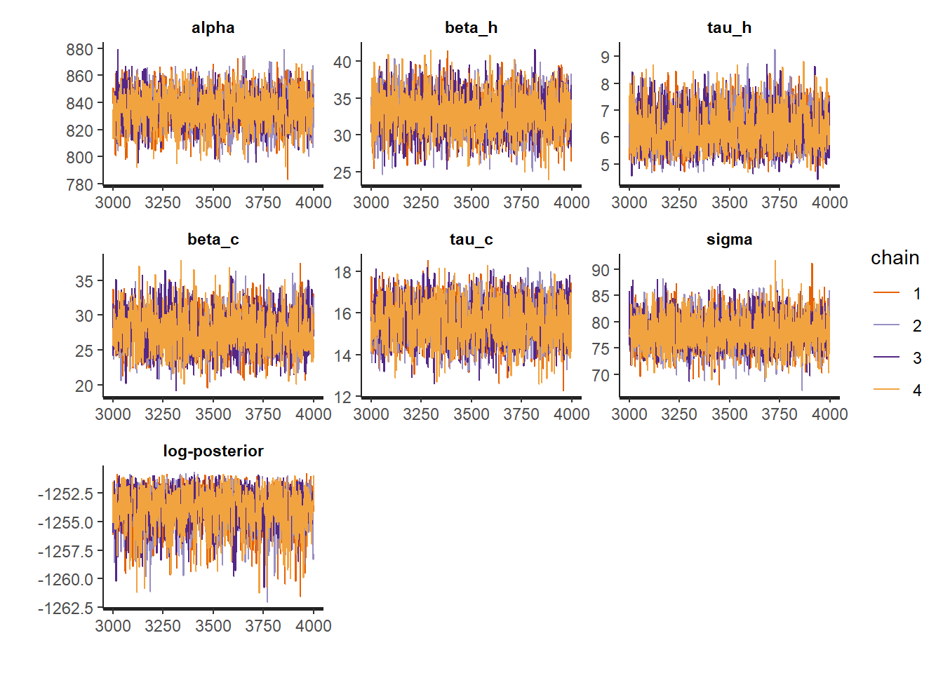
## Warning in par(usr): argument 1 does not name a graphical parameter

## Warning in par(usr): argument 1 does not name a graphical parameter

## Warning in par(usr): argument 1 does not name a graphical parameter

## Warning in par(usr): argument 1 does not name a graphical parameter

## Warning in par(usr): argument 1 does not name a graphical parameter

## Warning in par(usr): argument 1 does not name a graphical parameter

## Warning in par(usr): argument 1 does not name a graphical parameter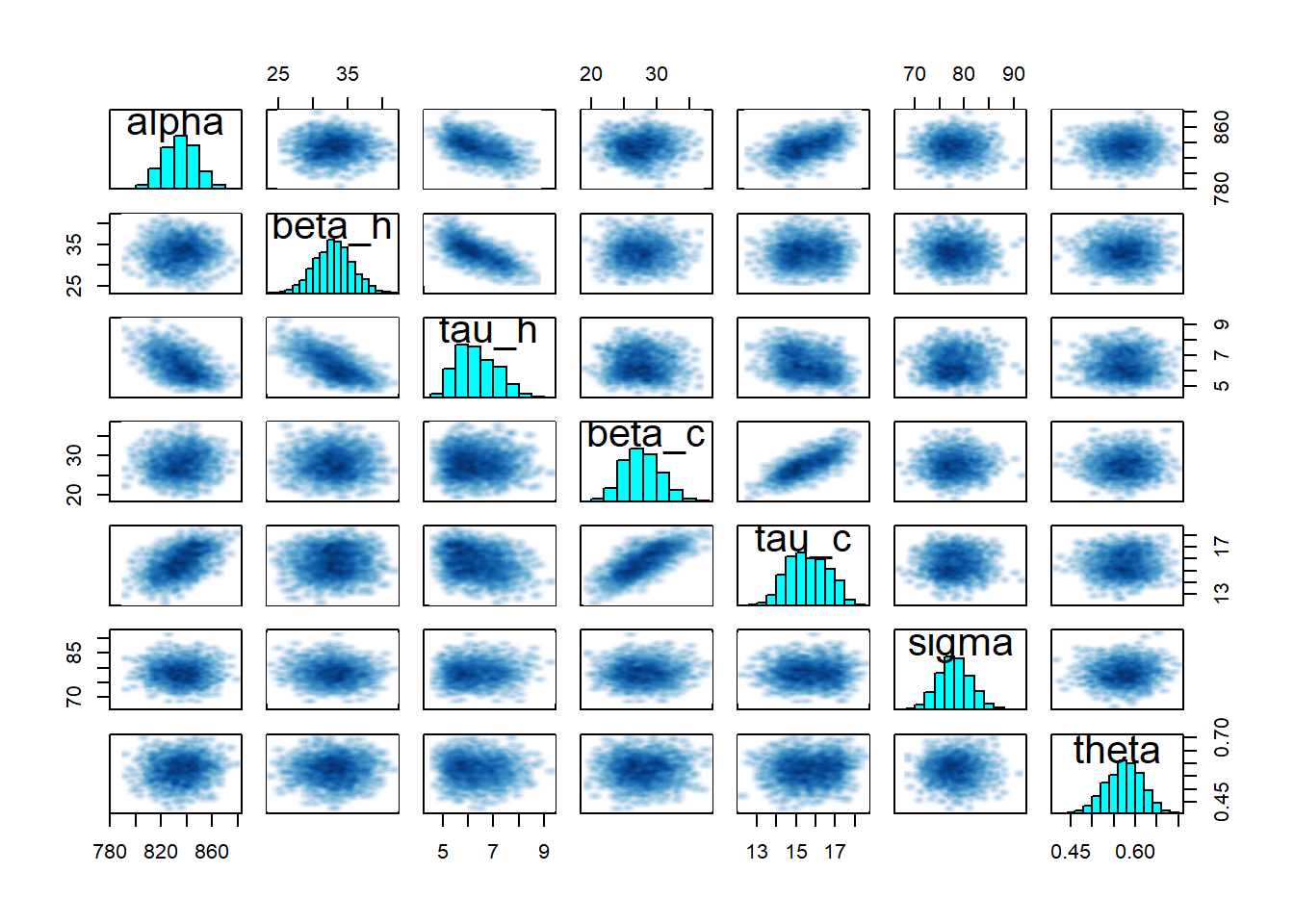
Remember that we need to validate our inference diagnostics criteria! All traces must match, n_eff should be in the thousands and Rhat exactly 1 for all parameters.
5.4.2 Model checking
The model checking metrics are the same as usual: coefficient of determination \(R^2\), CV(RMSE), F-statistic… Here we calculate them only from the mean prediction rather than the full posterior distribution.
la <- rstan::extract(fit, permuted = TRUE)
predict.mean <- colMeans(la$y_pre_pred)

residuals <- predict.mean - df.pre.day$E      # residuals
ssres <- sum(residuals^2)                     # sum of squared residuals
sstot <- sum((df.pre.day$E-mean(df.pre.day$E))^2) # total sum of squares

R2 <- 1 - ssres / sstot   # coefficient of determination
CVRMSE <- sqrt(ssres / nrow(df.pre.day)) / mean(df.pre.day$E)

print(paste("R2 =", R2))
print(paste("CV(RMSE) =", CVRMSE))
## [1] "R2 = 0.776975544980678"
## [1] "CV(RMSE) = 0.0795665214087723"The \(R^2\) has increased from 0.66 to 0.78 since we added the \(\mathrm{MA}(1)\) regression coefficient, and the CV(RMSE) has decreased. This suggests that the model better explains the data’s variance.
5.4.3 Savings
We choose to skip the prediction plot and go straight to the savings estimate and its confidence bounds:
##     2.5%      10%      50%      90%    97.5%
## 45397.71 47105.36 50212.43 53279.24 54963.14
Compared to the results of tutorial 2, the mean estimated savings are similar, but the uncertainty is about 10% larger.
5.4.4 Residuals
The whole point of this tutorial, compared to the previous one, is to reduce the autocorrelation of the prediction residuals, which would be a sign of a biased models and unreliable inferences. Have we succeded?
acf(residuals)
Figure 5.1: Autocorrelation function of prediction residuals
Every vertical line of this graph shows the correlation coefficient between the values of a series (here residuals) and its own values with a certain lag.
The lag-1 ACF has been significantly reduced. The cause for the correlation between consecutive residuals has not been solved, but the model now “knows” that something unexplained is causing it: predictions were made more uncertain as a way to aknowledge it.
We can zoom in on the lag-1 autocorrelation by plotting residuals versus their own previous value:
ggplot() +
  geom_point(mapping = aes(x=residuals, y=lag(residuals, n=1, default=0)))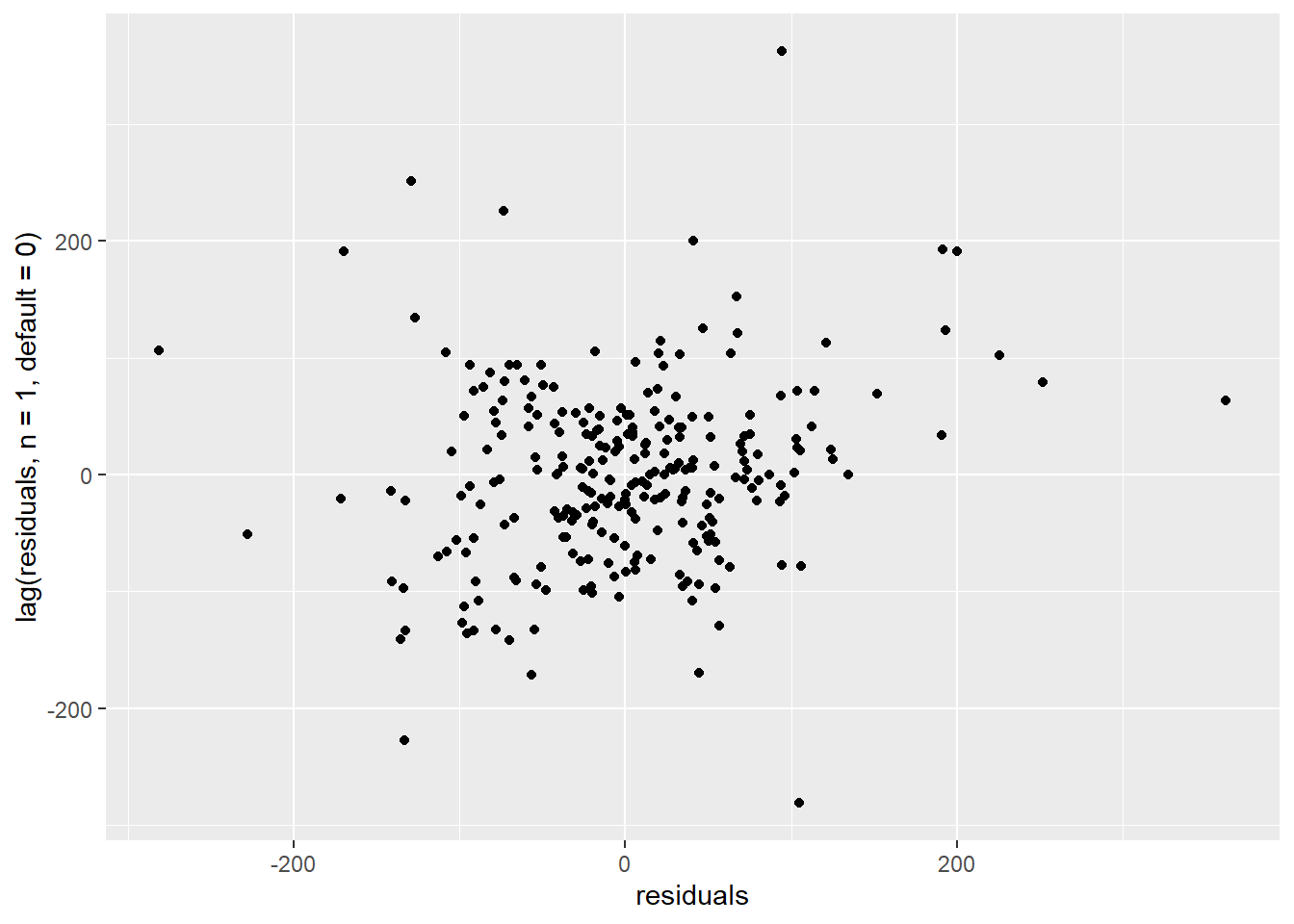
Figure 5.2: Correlation of consecutive residuals
There is no longer a visible trend on this scatter plot.
However, we can notice on Fig. @(fig:tuto3corr1) that some autocorrelation remains every 5 lags. Remember that since we filtered out week ends, each week of data comprises 5 measurements. Therefore, it looks like some weekly pattern has still not been properly captured.
ggplot() +
  geom_point(mapping = aes(x=residuals, y=lag(residuals, n=5, default=0)))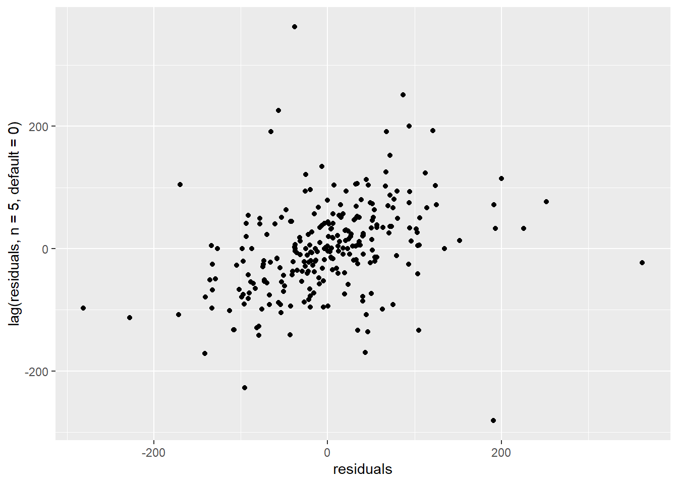
Figure 5.3: Correlation of residuals with lag-5
There is a trend here. We need to define a new model which includes regression terms for the lag-1 and lag-5 errors.
5.5 New model: MA(5)
5.5.1 Even more uncertainty
Fig. @(fig:tuto3corr1) suggests that our MA(1) change-point model still shows some autocorrelation after fitting, especially at lags 2 and 5. We are therefore tempted to extend it so that lag-5 residuals are predictors of the outcome variable \(y\):
\[\begin{align} y_n & = \alpha + \beta_{h}(\tau_{h}-x_n)^+ + \beta_{c}(x_n-\tau_{c})^+ + \theta_1 \varepsilon_{n-1} + \theta_5 \varepsilon_{n-5} + \varepsilon_n \tag{5.9} \\ \varepsilon_n & \sim \mathrm{normal}\left(0, \sigma\right) \tag{5.10} \end{align}\]
As we already stated, by doing so, we are not making the physical model \(f(x)=\alpha + \beta_{h}(\tau_{h}-x)^+ + \beta_{c}(x-\tau_{c})^+\) more complex. We are accounting for the fact that it does not completely explain the data on its own: \(y\) is explained by \(f\) plus something else. We can expect inferences from such a model to be more uncertain, but more reliable.
We call this model MA(5) because it is a fifth order moving average model, but we are not using all residuals up to lag 5; only lags 1 and 5. The Stan code for this model is in a separate file changepoint_ma15.stan, and is very similar to the previous model, MA(1).
The MA(5) model uses the same data as the MA(1) model we just fitted, so all we have to do is:
# Fitting the model
fit15 <- stan(
  file = 'models/changepoint_ma15.stan',  # Stan program
  data = model_data,        # named list of data
  chains = 4,               # number of Markov chains
  warmup = 3000,            # number of warmup iterations per chain
  iter = 4000,              # total number of iterations per chain
  cores = 2,                # number of cores (could use one per chain)
  refresh = 0,              # progress not shown
  control = list(max_treedepth = 12),
  seed = 5678,
)
You may notice some differences with the previous time we called the stan() function. This is because the MA(5) turned out to be much less identifiable than expected, and some precautions were required to reach convergence of all chains.
- Priors were included in the model itself
-
control = list(max_treedepth = 12)increases the maximum tree depth. It is mostly an efficiency measure. -
seedlets us specify the seed of the MCMC algorithm. I used it here because many attempts did not converge (non-matching chains), and I want to be able to show reproducible results on this page.
5.5.2 Results
After fitting, let’s find out if this new model is more reliable than the previous ones. The first model checking metric is the \(R^2\) coefficient:
la15 <- rstan::extract(fit15, permuted = TRUE) # all posterior variables
predict.mean <- colMeans(la15$y_pre_pred)     # mean prediction
residuals <- predict.mean - df.pre.day$E      # residuals
ssres <- sum(residuals^2)                     # sum of squared residuals
sstot <- sum((df.pre.day$E-mean(df.pre.day$E))^2) # total sum of squares
R2 <- 1 - ssres / sstot   # coefficient of determination
print(paste("R2 =", R2))
## [1] "R2 = 0.835995817169064"The \(R^2\) is now 0.84, which is significantly better than the original change-point model (0.66) and even the MA(1) model (0.78).
Now let’s look at the autocorrelation function of residuals:
acf(residuals)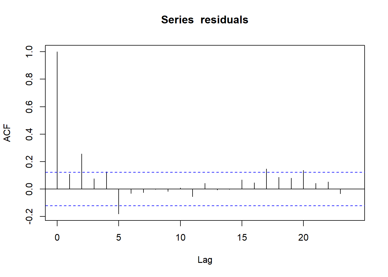 The ACF is now low enough for almost all lags. These metrics are reassuring: there is a good chance that we may trust the inferences from our fitted model. We can therefore proudly display our savings estimates, and their confidence bounds:
##     2.5%      10%      50%      90%    97.5%
## 39631.43 42487.19 47822.92 52811.51 55433.41
The 95% confidence interval of savings is now over 50% larger than from the MA(1) model, and nearly 80% larger than the original change-point model. This may sound like bad news, but it is more nuanced: this is the first model with completely reassuring model checking metrics. We can be much more confident that the real value of savings lies within these bounds.