2 Bayesian data analysis

This chapter only covers the basics of Bayesian inference, the motivation behind this choice and how to use it in practice. The internet has a lot of reading material on the matter if you wish to go further.

• Gelman et al’s book on Bayesian data analysis, aka The Big Bayesian Book, covers every aspect of this vast field and is very example-oriented.
• Bayesian workflow to data analysis is a practical summary, although still very comprehensive.
• Statistical rethinking is another vast Bayesian course spanning from theoretical fundamentals to practical examples.
• Michael Betancourt’s extensive lectures range from basics of probability theory to extremely detailed Bayesian workflow.

2.1 Motivation for a Bayesian M&V

Bayesian statistics are mentioned in the Annex B of the ASHRAE Guideline 14, after it has been observed that standard approaches make it difficult to estimate the savings uncertainty when complex models are required in a measurement and verification worflow:

“Savings uncertainty can only be determined exactly when energy use is a linear function of some independent variable(s). For more complicated models of energy use, such as changepoint models, and for data with serially autocorrelated errors, approximate formulas must be used. These approximations provide reasonable accuracy when compared with simulated data, but in general it is difficult to determine their accuracy in any given situation. One alternative method for determining savings uncertainty to any desired degree of accuracy is to use a Bayesian approach.”

Still on the topic of measurement and verification, and the estimation of savings uncertainty, several advantages and drawbacks of Bayesian approaches are described by (Carstens, Xia, and Yadavalli (2018)). Advantages include:

• Because Bayesian models are probabilistic, uncertainty is automatically and exactly quantified. Confidence intervals can be interpreted in the way most people understand them: degrees of belief about the value of the parameter.
• Bayesian models are more universal and flexible than standard methods. Models are also modular and can be designed to suit the problem. For example, it is no different to create terms for serial correlation, or heteroscedasticity (non-constant variance) than it is to specify an ordinary linear model.
• The Bayesian approach allows for the incorporation of prior information where appropriate.
• When the savings need to be calculated for “normalised conditions”, for example, a “typical meteorological year”, rather than the conditions during the post-retrofit monitoring period, it is not possible to quantify uncertainty using current methods. However, (Shonder and Im (2012)) have shown that it can be naturally and easily quantified using the Bayesian approach.

The first two points above are the most relevant to a data analyst: any arbitrary model structure can be defined to explain the data, and the exact same set of formulas can then be used to obtain any uncertainty after the models have been fitted.

2.2 Bayesian inference in theory

A Bayesian model is defined by two components:

• An observational model \(p\left(y|\theta\right)\), or likelihood function, which describes the relationship between the data \(y\) and the model parameters \(\theta\).
• A prior model \(p(\theta)\) which encodes eventual assumptions regarding model parameters, independently of the observed data. Specifying prior densities is not mandatory.

The target of Bayesian inference is the estimation of the posterior density \(p\left(\theta|y\right)\), i.e. the probability distribution of the parameters conditioned on the observed data. As a consequence of Bayes’ rule, the posterior is proportional to the product of the two previous densities:

\[\begin{equation} p(\theta|y) \propto p(y|\theta) p(\theta) \tag{2.1} \end{equation}\]

This formula can be interpreted as follows: the posterior density is a compromise between assumptions and evidence brought by data. The prior can be “strong” or “weak”, to reflect for a more or less confident prior knowledge. The posterior will stray away from the prior as more data is introduced.

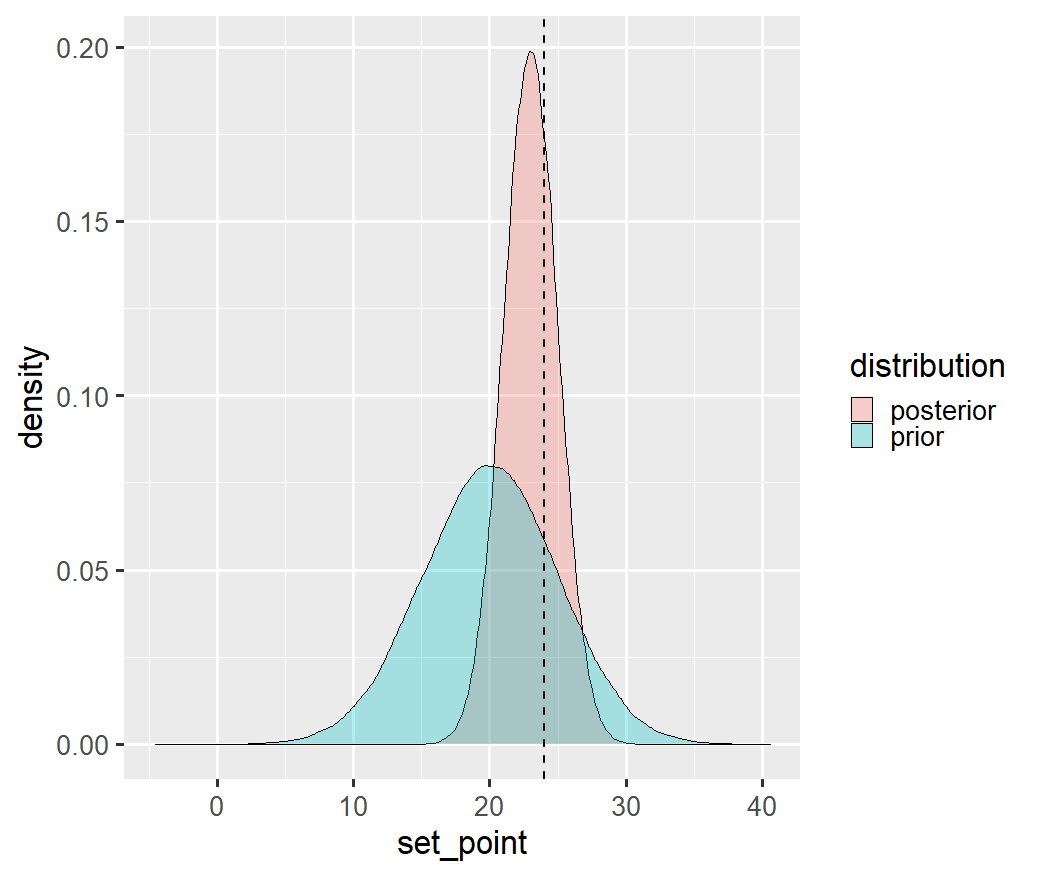
Figure 2.1: Example of estimating a set point temperature after assuming a Normal prior distribution centred around 20°C. The dashed line is the point estimate which would have been obtained if only the data had been considered. The posterior distribution can be seen as a “refinement” of the prior, given the evidence of the data.

In general, information from the posterior distribution is represented by summary statistics such as the mean, variance or credible intervals, which can be used to inform decisions and are easier to interpret than the full posterior distribution. Most of these summary statistics take the form of posterior expectation values of certain functions, \(f(\theta)\),

\[\begin{equation} \label{posterior_expectation} \mathbb{E}[f(\theta)] = \int p(\theta|y) f(\theta) \mathrm{d} \theta \tag{2.2} \end{equation}\]

More sophisticated questions are answered with expectation values of custom functions \(f(\theta)\). One common example is the posterior predictive distribution: in many applications, one is not only interested in estimating parameter values, but also the predictions \(\tilde{y}\) of the observable during a new period. The distribution of \(\tilde{y}\) conditioned on the observed data \(y\) is called the posterior predictive distribution:

\[\begin{equation} p\left(\tilde{y}|y\right) = \int p\left(\tilde{y}|\theta\right) p\left(\theta|y\right) \mathrm{d}\theta \tag{2.3} \end{equation}\]

The posterior predictive distribution is an average of the model predictions over the posterior distribution of \(\theta\). This formula is equivalent to the concept of using a trained model for prediction.

Apart from the possibility to define prior distributions, the main specificity of Bayesian analysis is the fact that all variables are encoded as probability densities. The two main results, the parameter posterior \(p(\theta|y)\) and the posterior prediction \(p\left(\tilde{y}|y\right)\), are not only point estimates but complete distributions which include a full description of their uncertainty.

2.3 A Bayesian data analysis workflow

This section is an excerpt of the author’s larger website on building energy statistical modelling.

2.3.1 Overview

As was mentioned in Sec. 1.3, inverse problems are all but trivial. It is possible that the available data is simply insufficient to bring useful inferences, but that we still try to train an unsuitable model with it. Statistical analysts need the right tools to guide model selection and training, and to warn them when there is a risk of biased inferences and predictions.

This chapter is an attempt to summarize the essential points of a Bayesian workflow from a building energy perspective. Frequentist inference is also mentioned, but as a particular case of Bayesian inference.

Gelman et al. (Gelman et al. (2013)) divide the process of Bayesian data analysis into three steps illustrated by Fig. 2.2:

1. Setting up a full probability model;
2. Conditioning on observed data (learning);
3. Evaluating the fit of the model and the implications of the resulting posterior (checking and validation).

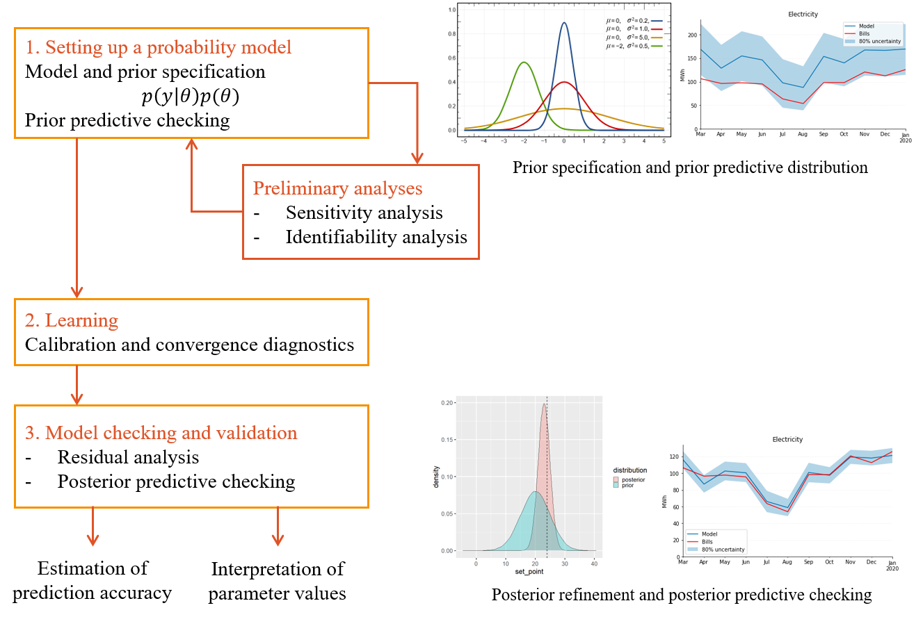
Figure 2.2: A workflow for the proper specification and training of one model. Most of the workflow is similar for frequentist and Bayesian inference.

2.3.2 Step 1: model specification

The first step into building our model is a conceptual analysis of the system and the available data. The first question is to decide what we want to learn from the data, and is related to the choice of measurement and modelling boundaries mentioned in Sec. 1.2, and the choice of model structure: which of the measurements is the dependent variable \(y\), which are the relevant explanatory variables \(x\), and how will the model parameters \(\theta\) be defined.

The model definition is greatly impacted by the time resolution and length of the dataset. Higher time resolutions (under an hour) enable the choice of dynamical models, which can encode more inferential information but imply a more complex development. Longer datasets (several months) enable the aggregation of data over longer resolutions and observations covering different weather conditions.

The next step is the development of the model: the translation of the conceptual narrative of the system into formal mathematical descriptions. The target is to formulate the entire system into probabilities that our fitting method can work with. In the case of simple regression models, the observational model may be summarized by a single likelihood function \(p(y|\theta)\), eventually conditioned on explanatory variables.

If the practitioner wishes to use a regression model to explain the relationship between the parameters and the data, doing so in a Bayesian framework is very similar to the usual (frequentist) framework. As an example, a Bayesian model for linear regression with three parameters \((\theta_0,\theta_1,\theta_2)\) and two explanatory variables \((X_1,X_2)\) may read: \[\begin{align} p(y|\theta,X) & = N\left(\theta_0 + \theta_1 X_1 + \theta_2 X_2, \sigma\right) \tag{2.4} \\ p(\theta_i) & = \Gamma(\alpha_i, \beta_i) \tag{2.5} \end{align}\]

This means that \(y\) follows a Normal distribution whose expectation is a linear function of \(\theta\) and \(X\), with standard deviation \(\sigma\) (the measurement error). The second equation is the prior model: in this example, each parameter is assigned a Gamma prior distribution parameterised by a shape \(\alpha\) and a scale \(\beta\). Other model structures can be formulated similarly: change-point models, polynomials, models with categorical variables… Bayesian modelling however allows for much more flexibility:

• Other distributions than the Normal distribution can be used in the observational model;
• Hierarchical modelling is possible: parameters can be assigned a prior distribution with parameters which have their own (hyper)prior distribution;
• Heteroscedasticity can be encoded by assuming a relationship between the error term and explanatory variables, etc.

More complex models with latent variables have separate expressions for the respective conditional probabilities of the observations \(y\), latent variables \(z\) and parameters \(\theta\). In this case, there is a likelihood function \(p(y,z|\theta)\) and a marginal likelihood function \(p(y|\theta)\) so that: \[\begin{equation} p(y|\theta) = \int p(y,z|\theta) \mathrm{d}z \tag{2.6} \end{equation}\]

The IPMVP option D relies on the use of calibrated building energy simulation (BES) models. These models are described by a much larger number of parameters and equations that the simple regression models typically used for other IPMVP options. In this context, it is not feasible to fully describe BES models in the form of a simple likelihood function \(p(y|\theta)\). In order to apply Bayesian uncertainty analysis to a BES model, it is possible to first approximate it with a Gaussian process (GP) model emulator. This process is denoted Bayesian calibration and was based on the seminal work of Kennedy and O’Hagan (Kennedy and O’Hagan (2001)). As opposed to the manual adjustment of building energy model parameters, Bayesian calibration explicitly quantifies uncertainties in calibration parameters, discrepancies between model predictions and observed values, as well as observation errors (Chong and Menberg (2018)).

2.3.3 Prior predictive checking

The full probability model is the formalization of many assumptions regarding the data-generating process. In theory, the model can be formulated only based on domain expertise, regardless of the data. In practice, a model which is inconsistent with the data has little chance to yield informative inferences after training. The prior predictive distribution, or marginal distribution of observations \(p(y)\), is a way to check for the consistency of our expertise.

\[\begin{equation} p\left(y\right) = \int p\left(y|\theta\right) p\left(\theta\right) \mathrm{d}\theta \tag{2.7} \end{equation}\]

Basically, computing this distribution is equivalent to running a few simulations of a numerical model before its training, with some assumed values of the parameters. In Bayesian terms, we first draw a finite number of parameter vectors \(\tilde{\theta}^{(m)}\) from the prior distribution, and use each of them to compute a model output \(\tilde{y}^{(m)}\):

\[\begin{align} \tilde{\theta}^{(m)} & \sim p(\theta) \tag{2.8} \\ \tilde{y}^{(m)} & \sim p(y|\tilde{\theta}^{(m)}) \tag{2.9} \end{align}\]

This set of model outputs approximates the prior probability distribution. If large inconsistencies can be spotted between this distribution and measurements, we can adjust some assumptions regarding the prior definition or the structure of the observational model. An example of prior predictive checking is shown on the top right of Fig. 2.2, which suggests a model structures which does not contradict the observations.

2.3.4 Step 2: computation with Markov Chain Monte Carlo

Except in a few convenient situations, the posterior distribution is not analytically tractable. In practice, rather than finding an exact solution for it, it is estimated by approximate methods. The most popular option for approximate posterior inference are Markov Chain Monte Carlo (MCMC) sampling methods. When it is not possible or not computationally efficient to sample directly from the posterior distribution, Markov Chain simulation is used to stochastically explore the typical set, i.e. the regions of parameter space which have a significant contribution to the desired expectations. Markov chains used in MCMC methods are designed so that their stationary distribution is the posterior distribution. If the chain is long enough, the state history of the chain provides samples from the typical set \(\left(\theta^{(1)},...,\theta^{(S)}\right)\) \[\begin{equation} \theta^{(s)} \sim p(\theta | y) \tag{2.10} \end{equation}\] where each draw \(\theta^{(s)}\) contains a value for each of the parameters of the model.

This guide does not aim at explaining MCMC algorithms and their characteristics, but we may refer to this paper (Betancourt (2017)) for a description of the state-of-the-art Hamiltonian Monte Carlo alogrithm.

Posterior expectation values can be accurately estimated by Monte Carlo estimator. Based on exact independent random samples from the posterior distribution \(\left(\theta^{(1)},...,\theta^{(S)}\right) \sim p(\theta | y)\), the expectation of any function \(f(\theta)\) can be estimated with \[\begin{equation} \mathbb{E}[f(\theta)] \approx \frac{1}{N} \sum_{n=1}^{N} f(\theta)^{(n)} \tag{2.11} \end{equation}\]

Markov Chain Monte Carlo estimators converge to the true expectation values as the number of draws approaches infinity. In practice, diagnostics must be applied to check that the estimator follows the central limit theorem, which ensures that the estimator is unbiased after a finite number of draws. For that purpose it is first recommended to compute the (split-)\(\hat{R}\) statistic, or Gelman-Rubin statistic, with multiple chains initialized at different initial positions and split into two halves (Gelman et al. (2013)). The \(\hat{R}\) statistic measures for each scalar parameter, \(\theta\), the ratio of samples variance within each chain \(W\) to the sample variance of all combined chains \(B\),

\[\begin{equation} \hat{R} = \sqrt{\frac{1}{W} \left(\frac{N-1}{N}W + \frac{1}{N}B \right)} \tag{2.12} \end{equation}\]

where \(N\) is the number of samples. If the chains have not converged, \(W\) will underestimate the variance, since the individual chains have not had time to range all over the stationary distribution, and \(B\) will overestimate the variance, since the starting positions were chosen to be overdispersed.

Another important convergence diagnostics tool is the effective sample size (ESS), defined as:

\[\begin{equation} \text{ESS} = \frac{N}{1 + 2 \sum_{l=1}^{\infty} \rho_l} \tag{2.13} \end{equation}\]

with \(\rho_l\) the lag-\(l\) autocorrelation of a function \(f\) over the history of the Markov chain. The effective sample size is an estimate of the number of independent samples from the posterior distribution.

The diagnostic tools introduced in this section provide a principled workflow for reliable Bayesian inferences. They are readily available in most Bayesian computation libraries. Based on the recent improvements to the \(\hat{R}\) statistic (Vehtari et al. (2021)), it is recommended to use the samples only if \(\hat{R} < 1.01\) and \(\text{ESS} > 400\).

2.3.5 Step 3: model checking and validation

After model specification and learning, the third step of the workflow is model checking and validation. It should be conducted before any conclusions are drawn, and before the prediction accuracy of the model is estimated.

• The posterior predictive distribution

The basic way of checking the fit of a model to data is to draw simulated values from the trained model and compare them to the observed data. In a non-Bayesian framework, we would pick the most likely point estimate of parameters, such as the maximum likelihood estimate, use it to compute the model output \(\hat{y}\), and conduct residual analysis. In a Bayesian framework, posterior predictive checking allows some more possibilities.

The posterior predictive distribution is the distribution of the observable \(\tilde{y}\) (the model output) conditioned on the observed data \(y\): \[\begin{equation} p\left(\tilde{y}|y\right) = \int p\left(\tilde{y}|\theta\right) p\left(\theta | y\right) \mathrm{d}\theta \tag{2.14} \end{equation}\] This definition is very similar to the prior predictive distribution given in Sec. 2.3.3, except that the prior \(p(\theta)\) has been replaced by the posterior \(p(\theta|y)\). Similarly, it is simple to compute if the posterior has been approximated by an MCMC procedure: we first draw a finite number of parameter vectors \(\theta^{(m)}\) from the posterior distribution, and use each of them to compute a model output \(\tilde{y}^{(m)}\): \[\begin{align} \theta^{(m)} & \sim p(\theta|y) \tag{2.15}\\ \tilde{y}^{(m)} & \sim p(y|\theta^{(m)}) \tag{2.16} \end{align}\] This set of model outputs approximates the posterior probability distribution.

The following methods of model checking may apply to either a frequentist or a Bayesian framework.

• If the fitting returns a point estimate of parameters \(\hat{\theta}\), then a single profile of model output \(\hat{y}\) can be calculated from it, either to be compared with the training data set \(y_\mathit{train}\) or to a separate test data set \(y_\mathit{test}\).

• If the fitting returns a posterior distribution \(p(y|\theta)\), the same comparisons may be applied to any of the \(\tilde{y}^{(m)}\) samples.

• Measures of model adequacy

After fitting, either ordinary linear regression or more sophisticated ones, some metrics may assess the predictive accuracy of the model.

• The R-squared (\(R^2\)) index is the proportion of the variance of the dependent variable that is explained by the regression model (closest to 1 is better)

\[\begin{equation} R^2 = 1-\frac{\sum_{i=1}^N\left(y_i - \hat{y}_i\right)^2}{\sum_{i=1}^N\left(y_i - \bar{y}_i\right)^2} \tag{2.17} \end{equation}\]

• The root-mean-square-error (RMSE) simply measures the differences between model predictions \(\hat{y}\) and observations \(y\) (lower is better)

\[\begin{equation} \mathrm{CV(RMSE)} = \frac{1}{\bar{y}} \sqrt{\frac{\sum_{i=1}^N\left(\hat{y}_i-y_i\right)^2}{N}} \tag{2.18} \end{equation}\]

• Coverage Width-based Criterion (CWC) (Chong, Augenbroe, and Yan (2021)), an indicator for probabilistic forecasts which measures the quality of the predictions based on both their accuracy and precision.

The \(R^2\) and CV-RMSE indices are too often treated as validation metrics. If they are calculated using a test data set, they can indeed estimate the model predictive ability outside of the training data set. They however do not ensure that the model correctly captures the data generating process: this is what residual analysis is for.

• Residual analysis

The hypothesis of an unbiased model assumes that the difference between the model output and the observed temperature is a sequence of independent, identically distributed variables following a Gaussian distribution with zero mean and constant covariance. In the example of a linear regression model, this condition may read: \[\begin{equation} r_i = y_i - \left( \hat{\theta}_0 + \hat{\theta}_1 X_{i,1} + \hat{\theta}_2 X_{i,2} \right) \sim N(0,\sigma) \tag{2.19} \end{equation}\] where \(r_i\) are the prediction residuals. Residual analysis is the process of checking the validity of their four hypotheses (independence, identical distribution, zero mean, constant variance), and the main step of model validation. It allows identifying problems that may arise after fitting a regression model (James et al. (2013)), among which: correlation of error terms, outliers, high leverage points, colinearity…

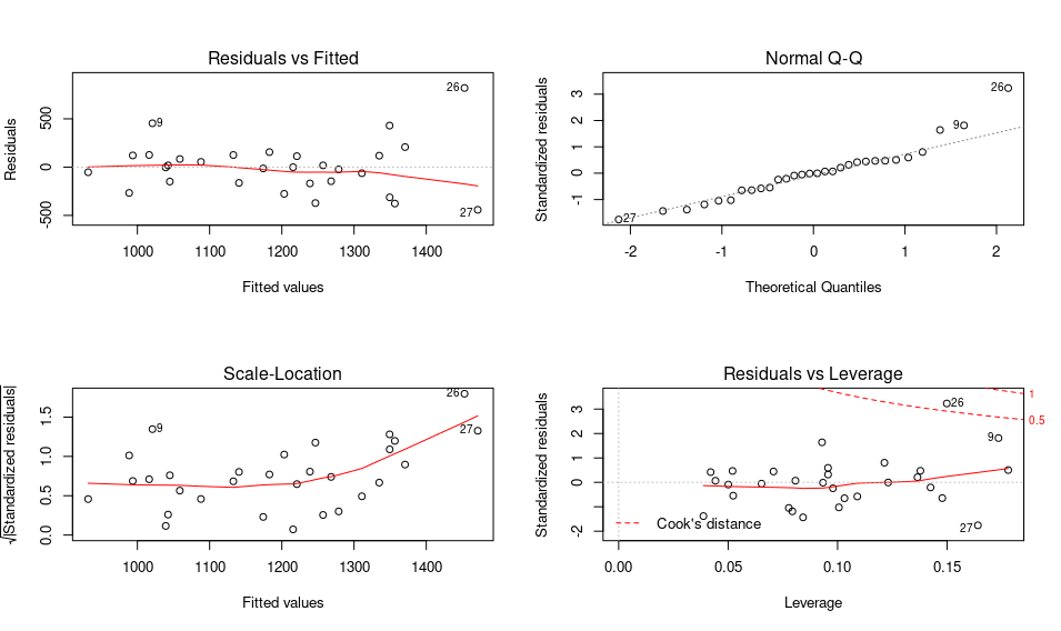
Figure 2.3: Example of residual plots after an ordinary linear regression in R: fitted vs residuals, Q-Q plot, scale location and residuals vs leverage

Residual analysis can be performed by an array of tests and graphs, some of which are shown on Fig. 2.3.

• A simple plot of the residuals versus the model output should not display any trend. The same goes for a plot of residuals vs any of the explanatory variables. Should a trend be visible, the model structure is probably insufficient to explain the data.
• A quantile-quantile (Q-Q) plot (upper right) is a way to check if the distribution of residuals is approximately Gaussian
• The scale-location plot (lower left) is a way to check the hypothesis of homoskedasticity, i.e. constant variance
• The residuals vs leverage plot (lower right) allows identifying eventual outliers and high leverage points.

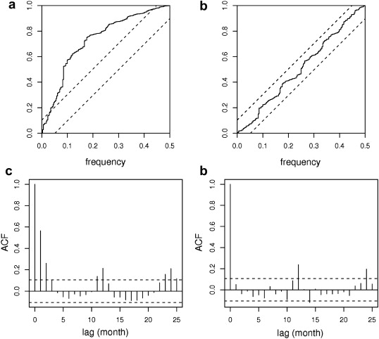
Figure 2.4: Autocorrelation function (top) and cumulated periodogram (bottom) of an insufficient model (left) and a sufficient model (right)

Most importantly, the correlation among the error terms should be checked. The autocorrelation function (ACF) checks the independence of residuals and may reveal lag dependencies which suggest influences that the model does not properly take into account. This is particularly important for time series models, and therefore well explained the time series litterature (Shumway and Stoffer (2000)). Alternatively, the Durbin-Watson test quantitatively checks for autocorrelation in regression models. “If there is correlation among the error terms, then the estimated standard errors will tend to underestimate to true standard errors. As a result, confidence and prediction intervals will be narrower than they should be.”(James et al. (2013))

If residuals display unequal variances or correlations, then the inferences and predictions of the fitted model should not be used. The model should be modified and re-trained according to the practitioner’s expertise and diagnostics of the analysis: additional explanatory variables can be included if possible.

2.4 Bayesian M&V in practice

2.4.1 Estimating savings and their uncertainty

The following workflows for M&V can be followed regardless of the chosen type of model (regression model for options A, B and C, or GP emulator for option D). The choice of workflow will mostly depend on the availability of data during the baseline and reporting periods.

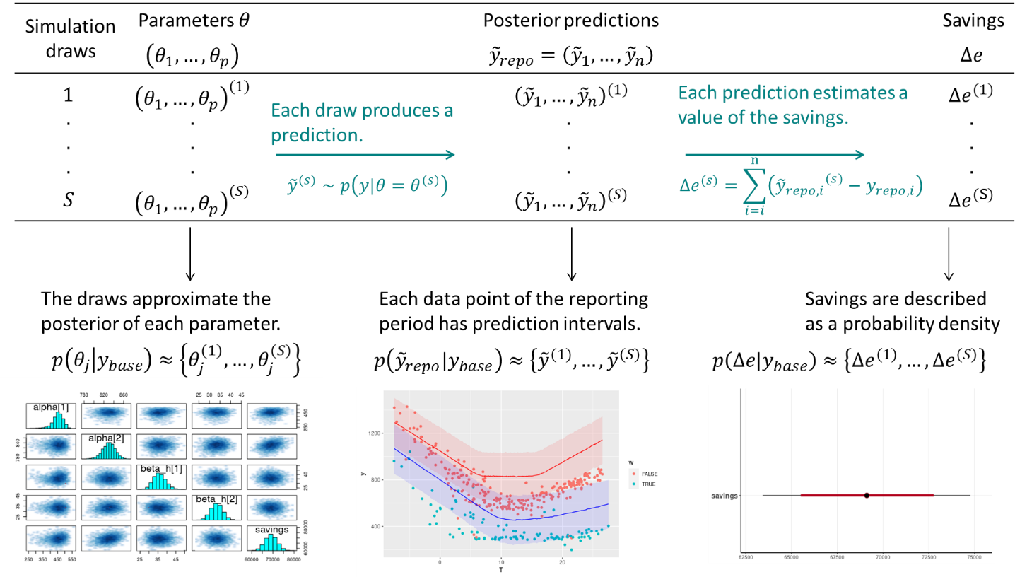
Figure 2.5: Estimation of savings with uncertainty in an avoided consumption workflow. The step of model validation is not displayed.

Here is a summary of the workflow to estimate savings and their uncertainty, when following the reporting period basis, or avoided energy consumption. We assume that the measurement boundaries have been defined and that data \(y_\mathit{base}\) and \(y_\mathit{repo}\) have been recorded during the baseline and reporting period respectively.

• As with standard approaches, choose a model structure to describe the data with, and formulate it as a likelihood function. Formulate eventual “expert knowledge” assumptions in the form of prior probability distributions.
• Run a MCMC (or other) algorithm to obtain a set of samples \(\left(\theta^{(1)},...,\theta^{(S)}\right)\) which approximates the posterior distribution of parameters conditioned on the baseline data \(p\left(\theta | y_\mathit{base}\right)\). Validate the inference by checking convergence diagnostics: R-hat, ESS, etc.
• Validate the model by computing its predictions during the baseline period \(p\left(\tilde{y}_\mathit{base} | y_\mathit{base}\right)\). This can be done by taking all (or a representative set of) samples \(\theta^{(s)}\) individually, and running a model simulation \(\tilde{y}_\mathit{base}^{(s)} \sim p\left(y_\mathit{base} | \theta=\theta^{(s)}\right)\) for each. This set of simulations generates the posterior predictive distribution of the baseline period, from which any statistic can be derived (mean, median, prediction intervals for any quantile, etc.). The measures of model validation (R-squared, net determination bias, t-statistic…) can then be computed either from the mean, or from all samples in order to obtain their own probability densities.
• Compute the reporting period predictions in the same discrete way: each sample \(\theta^{(s)}\) generates a profile \(\tilde{y}_\mathit{repo}^{(s)} \sim p\left(y_\mathit{repo} | \theta=\theta^{(s)}\right)\), and this set of simulations generates the posterior predictive distribution of the reporting period.
• Since each reporting period prediction \(\tilde{y}_\mathit{repo}^{(s)}\) can be compared with the measured reporting period consumption \(y_\mathit{repo}\), we can obtain S values for the energy savings, which distribution approximate the posterior probability of savings.

\[\begin{align} \Delta e^{(s)} & = \sum_{i=1}^n\left(\tilde{y}_\mathit{repo}^{(s)}(i)-y_\mathit{repo}(i)\right) \tag{2.19} \\ & \sim p\left(\Delta e | y_\mathit{base}, y_\mathit{repo}\right) \tag{2.20} \end{align}\]

In a normalised savings workflow, a numerical model is trained on both the baseline and the reporting period data. Each trained model then predicts the energy consumption during a period of normalised conditions, and savings are estimated by comparing these predictions.

• Two posterior distributions should be produced \(\left(\theta^{(1)},...,\theta^{(S)}\right)_\mathit{base}\) and \(\left(\theta^{(1)},...,\theta^{(S)}\right)_\mathit{repo}\), in a similar way that a model is trained for each period. The validation metrics of each model should be checked using the posterior predictions of their own training period.

• Each model computes a set of \(S\) posterior predictions during the normalised period, by sampling from its parameter posterior distribution: \[\begin{align} \tilde{y}_{\mathit{norm}|\mathit{base}}^{(s)} \sim p\left(y_\mathit{norm} | \theta=\theta_\mathit{base}^{(s)}\right) \tag{2.21}\\ \tilde{y}_{\mathit{norm}|\mathit{repo}}^{(s)} \sim p\left(y_\mathit{norm} | \theta=\theta_\mathit{repo}^{(s)}\right)\tag{2.22} \end{align}\]

• We can obtain \(S\) values of the savings from these \(S\) pairs of predictions: \[\begin{equation} \Delta e^{(s)} = \sum_{i=1}^n\left(\tilde{y}_{\mathit{norm}|\mathit{base}}^{(s)}(i) - \tilde{y}_{\mathit{norm}|\mathit{repo}}^{(s)}(i)\right) \tag{2.23} \end{equation}\]

2.4.2 Software tools

The rest of this guide is a series of tutorials so that the reader may see these methods in practice. Unlike classical regression, the modelling part requires stepping out of Excel spreadsheets and using a dedicated computing environment.

We use the Stan platform for statistical modelling. Its algorithms are accessible through interfaces into most scientific computing languages: Python, R, Julia, Matlab…

The majority of Stan users seem to favor the R language, hence this choice in our tutorials. As an alternative to full Stan models, rstanarm is an R package for “people who would be open to Bayesian inference if using Bayesian software were easier but would use frequentist software otherwise”

For Python users, PyMC and Pyro are popular Bayesian modelling alternatives. Julia users may use Turing. The Stan models we propose can still be interfaced with these two languages.

Additionally, specialised plotting libraries were made for exploratory analysis of Bayesian models. We recommend users to give them a try:

• The bayesplot R package for Stan models;
• The ArviZ package for Python and Julia.