3 Tutorial 1: linear regression and introduction to Stan

This first tutorial serves as an introduction to the Stan platform, and shows that Bayesian analysis obtains the same uncertainty assessments as classical methods, when analytical solutions are available.

For this purpose, we use a very short dataset and an ordinary linear regression model.

3.1 Data

The data are monthly measurements of whole-facility energy use (kWh), as well as heating degree-days and cooling degree-days (°C.day).

library(rstan)
library(tidyverse)

# Baseline data: cooling and heating degree days, energy use
df.pre <- data.frame(cdd = c(0, 10, 15, 21, 21, 14, 0, 0, 0, 0, 0, 0),
                     hdd = c(14, 0, 0, 0, 0, 0, 2, 20, 18, 32, 27, 20),
                     use = c(35936, 22260, 20970, 25438, 28547, 24394,
                             24224, 38767, 42205, 49649, 43540, 43734))
# Reporting period data: cooling and heating degree days, energy use
df.post <- data.frame(cdd = c(0, 3, 13, 23, 19, 16, 0, 0, 0, 0, 0, 0),
                      hdd = c(5, 0, 0, 0, 0, 0, 2, 19, 20, 24, 25, 14),
                      use = c(25416, 17445, 13626, 19295, 17970, 15158,
                              13293, 35297, 35665, 38562, 33383, 37244))

ggplot() +
  geom_point(data = df.pre, aes(x=hdd, y=use), color="blue") +
  geom_point(data = df.post, aes(x=hdd, y=use), color="red")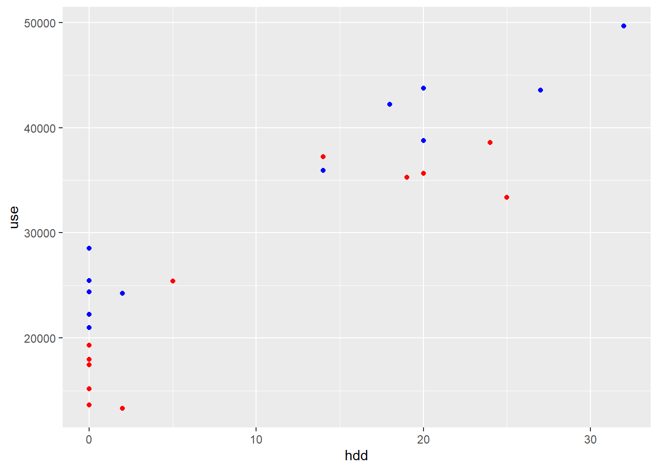

Figure 3.1: Electricity use vs. heating degree days; blue: pre-ECM; red: post-ECM

3.2 Model specification: first look at a Stan model

3.2.1 Ordinary linear regression

After a quick look at the data, we can assume a linear relationship between the dependent variable (energy use) and both explanatory variables (hdd and cdd).

I wrote a longer lecture on ordinary linear regression here. We don’t differentiate between simple and multiple regression, i.e. models with one or several explanatory variable, since they are solved the same way.

We consider a dependent variable $y$, and a set of $k$ explanatory (independent) variables $x=(x_1,...,x_k)$, and assume that a series of $n$ values of each have been measured. We therefore have a vector $\mathbf{y}=\left\{y_i\right\}_{i=1}^n$ and a matrix $X = \left\{x_{i1},...x_{ik}\right\}_{i=1}^n$ of dependent and independent variable measurements.

The ordinary linear regression model states that the distribution of each $y_i$ given the predictors $\mathbf{X}_i$ is normal with a mean that is a linear function: \[\begin{align} y_i & = \alpha + \beta_1 x_{i1} + ... + \beta_k x_{ik} + \varepsilon_i \tag{3.1} \\ \varepsilon_i & \sim \mathrm{normal}(0, \sigma) \tag{3.2} \end{align}\] or in matrix form: \[\begin{equation} \mathbf{y} = \alpha + \mathbf{X} \cdot \mathbf{\beta} + \mathbf{\varepsilon} \tag{3.3} \end{equation}\] The parameters $(\alpha, \beta_1, ..., \beta_k, \sigma)$ are a vector of coefficients to be determined. Ordinary linear regression assumes a normal linear model in which observation errors $\varepsilon_i$ are independent and have equal variance $\sigma^2$ (hypothesis of homoscedasticity).

3.2.2 Linear regression with Stan

Linear regression is naturally the first example given in the Stan documentation. The following model has been extended a bit for the purpose of our study.

A Stan model can be either written in a separate file, or included into your R script (or other language) as follows:

linearregression <- "
data {
// Baseline data (pre)
  int<lower=0> N;     // number of data items
  int<lower=0> K;     // number of predictors
  matrix[N, K] x;     // predictor matrix
  vector[N] y;        // outcome vector
// Reporting period data (post)
  int<lower=0> N_post;  // number of data items
  matrix[N, K] x_post;     // predictor matrix
  vector[N] y_post;        // outcome vector
}
parameters {
  real alpha;           // intercept
  vector[K] beta;       // coefficients for predictors
  real<lower=0> sigma;  // error scale
 }
model {
  y ~ normal(alpha + x * beta, sigma);  // likelihood
}
generated quantities {
  vector[N] predict_pre;
  vector[N_post] predict_post;
  real savings = 0;
  
  for (n in 1:N) {
    predict_pre[n] = normal_rng(x[n] * beta + alpha, sigma);
  }
  
  for (n in 1:N_post) {
    predict_post[n] = normal_rng(x_post[n] * beta + alpha, sigma);
    savings += predict_post[n] - y_post[n];
  }
}
"

The code is made of several blocks delimited by braces. There are up to seven types of blocks in a Stan model, but we only used four here. Their order is important in the code, but we describe them here in another order:

The model block is the center of the Stan code. This is where we declare the model that relates the dependent variable $y$ (energy use) to the explanatory variables $x$ (heating and cooling degree-days):

model {
  y ~ normal(alpha + x * beta, sigma);
}

This line states that we expect $y$ to be normally distributed around the linear function $\alpha + \mathbf{X} \cdot \mathbf{\beta}$, with standard deviation $\sigma$. It is identical to Eq. (3.3).

The data block contains the definition of the data to be passed to the model. The variables declared in this block are the arguments that the model will use: the vector $\mathbf{y}$ and matrix $\mathbf{X}$ for each of the “pre” and “post” periods. The number of data items is also a requirement, since it is used as a variable by the Stan model.
The parameters block declares the variables that will be learned by model training: the intercept $\alpha$, the slopes $\beta$ and the noise scale $\sigma$.
The generated quantities block is optional and does not influence model training. It is used to evaluate any function of the parameters $f(\theta)$ at every sample, so that we may directly obtain its posterior distribution $p(f(\theta)|y)$ (see Eq. (2.11)). Two variables are computed here:
- predict_pre and predict_post are the model’s prediction of energy use during the pre and post-ECM periods. They use the parameter models $(\alpha, \beta, \sigma)$ learned with pre-retrofit data, and matrix of dependent variables for each period.
- savings is the total difference between measured and predicted post-retrofit energy use. By including these two variables in the generated quantities block.

3.3 Model fit and inference diagnostics

3.3.1 Sampling from the posterior

The next step is to map the data contained in the df.pre and df.post dataframes to the Stan model. We do this by defining a list of variables that should match all items defined in the data block:

data_list <- list(N = nrow(df.pre),
                  K = 2,
                  x = df.pre %>% select(cdd, hdd),
                  y = df.pre$use,
                  N_post = nrow(df.post),
                  x_post = df.post %>% select(cdd, hdd),
                  y_post = df.post$use)

The first column of the $\mathbf{X}$ matrix are the cooling degree-days, and the second column are the heating degree-days.

We can now get a fit with the following command. The important arguments are:

model_code points to the Stan code. If you chose to write the R code in a separate file, for instance called linearregression.stan, you may replace the line model_code = linearregression with file = 'linearregression.stan' (by pointing to the appropriate location of the file).
data points to the list of variables that we just defined.
chains should be at least 4.
iter is the number of iterations per chain.
warmup is the number of discarded iterations at the start of every chain. Default values are chains = 4, warmup = 1000 and iter = 2000, which will result in chains*(iter-warmup)=4000 samples. This appeared slightly insufficient in our case because of the very small dataset, so we raised iter.

fit <- stan(
  model_code = linearregression,  # Stan program
  data = data_list,        # named list of data
  chains = 4,               # number of Markov chains
  warmup = 1000,            # number of warmup iterations per chain
  iter = 3000,              # total number of iterations per chain
  cores = 2,                # number of cores (could use one per chain)
  refresh = 0,              # progress not shown
)

Model fitting takes longer the first time the stan() command is run, because the model must first be compiled. This compilation is however only required once per model, which means running it again with new data is faster.

3.3.2 Results

The fit object returned by stan is associated with methods such as print, plot and pairs, letting us have a first look at our results.

The print method shows some posterior metrics of the parameters and generated quantities: mean, standard deviation, quantiles, effective sample size, R-hat.

print(fit, pars=c("alpha", "beta", "sigma", "savings"), probs=c(.025,.5,.975))

## Inference for Stan model: anon_model.
## 4 chains, each with iter=3000; warmup=1000; thin=1; 
## post-warmup draws per chain=2000, total post-warmup draws=8000.
## 
##             mean se_mean       sd     2.5%      50%     97.5% n_eff Rhat
## alpha   22869.14   56.85  2566.67 17778.70 22854.90  28107.04  2038    1
## beta[1]   115.60    3.67   173.61  -226.77   117.47    465.08  2239    1
## beta[2]   872.38    2.65   124.44   617.87   873.58   1124.87  2201    1
## sigma    3132.76   20.49   914.82  1905.86  2939.05   5517.54  1993    1
## savings 75696.75  203.12 16375.91 43296.92 75768.33 107740.79  6500    1
## 
## Samples were drawn using NUTS(diag_e) at Tue Jun 20 14:18:48 2023.
## For each parameter, n_eff is a crude measure of effective sample size,
## and Rhat is the potential scale reduction factor on split chains (at 
## convergence, Rhat=1).

traceplot shows the traces of the selected parameters and variables. If the fitting has converged, all traces should coincide and approximate posterior distributions.

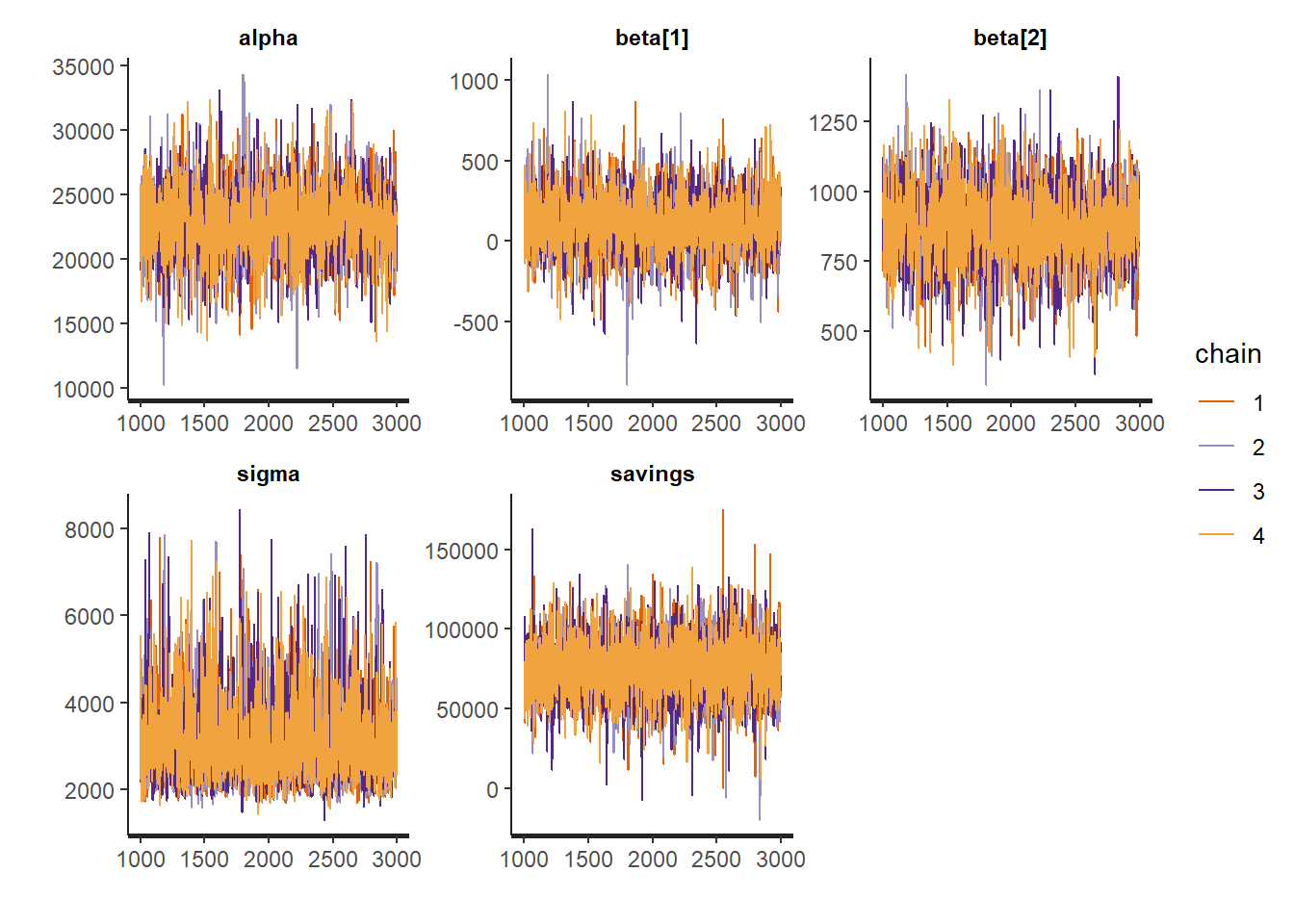
traceplot(fit, pars=c("alpha", "beta", "sigma", "savings"))

Figure 3.2: Traces of the regression coefficients

pairs shows the pairwise relationships between parameters. Strong interactions between some parameters are an indication that the model should be re-parameterised.

pairs(fit, pars=c("alpha", "beta", "sigma", "savings"))

## Warning in par(usr): argument 1 does not name a graphical parameter

## Warning in par(usr): argument 1 does not name a graphical parameter

## Warning in par(usr): argument 1 does not name a graphical parameter

## Warning in par(usr): argument 1 does not name a graphical parameter

## Warning in par(usr): argument 1 does not name a graphical parameter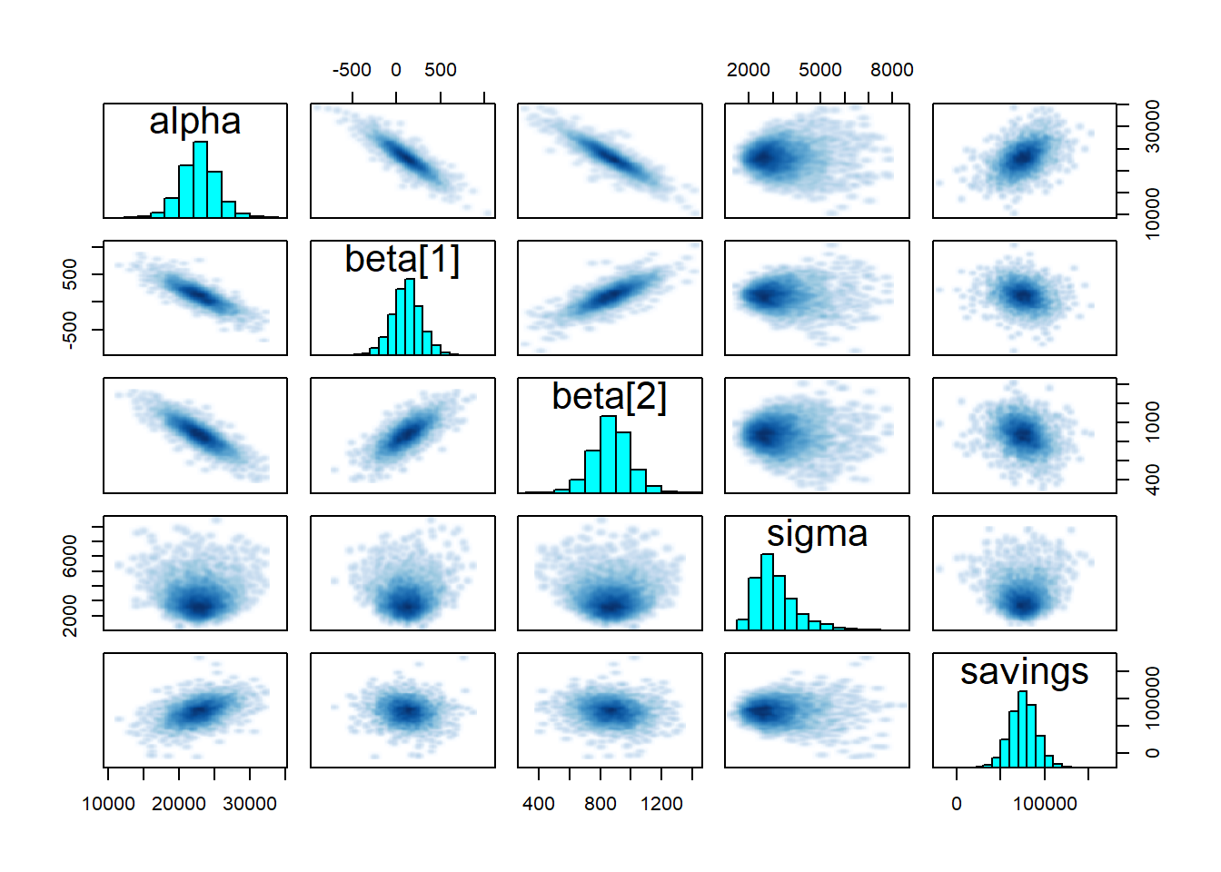

Figure 3.3: Pairplot of the regression coefficients

3.3.3 Inference diagnostics

Running the stan() command may return a variety of warnings to help users diagnose and resolve underlying modelling problems.

In order to draw reliable inferences from our results, we need at least a few green lights:

High enough effective sample size (ESS) for all parameters (seen on the table shown by print);
R-hat lower than 1.01, to ensure that chains have converged;
No remaining warnings about BFMI (Bayesian fraction of missing information), divergent transitions or maximum treedepth.

Some of these criteria may seem obscure to new users of Bayesian computation, but they should not be ignored. This guide suggests ways to solve problems. This is part of a larger workflow of model building, testing and critique/evaluation.

The first thing to try when traces have not converged is to increase warmup and iterations. This may be enough to get better ESS and R-hat
There are some possible “hidden” adjustments to the MCMC algorithm to solve some warnings (see this example)

fit <- stan(...
            control = list(adapt_delta = 0.99, stepsize = 0.01, max_treedepth = 15)
)

If problems remain, it might be a sign of model inadequacy. The solution is then to reduce the model and use stronger priors, as the data may not be sufficient to inform all parameters.

Diagnostics may be facilitated by the use of specialised plotting libraries made for exploratory analysis of Bayesian models:

The bayesplot R package
The ArviZ package for Python and Julia has methods dedicated to inference diagnostics

3.4 Model checking and validation

3.4.1 Measures of model adequacy

MCMC convergence is necessary, but does not guarantee that our model is the best choice for our case! Assessing the adequacy of the fitted model is just as necessary in a Bayesian framework as with classical frequentist methods.

The extract function returns model parameters and generated quantities into a named list.

la <- rstan::extract(fit, permuted = TRUE)
summary(la$savings)

##    Min. 1st Qu.  Median    Mean 3rd Qu.    Max. 
##  -19933   65558   75768   75697   85640  174954

For instance la$alpha and la$savings hold the value of the parameter $\alpha$ and the estimated savings for each of our many samples (in the example above, we have $N_s=8000$ samples). Similarly, la$prediction is a $N_s\times 12$ matrix because we have $N_s$ samples of each predicted energy use.

Here is a way to summarise posterior predictions into only a few quantiles:

# median, lower and upper bounds of the 95% prediction intervals
predict.pre <- apply(la$predict_pre, 2, quantile, probs=c(0.025, 0.5, 0.975))
# mean prediction
predict.mean <- colMeans(la$predict_pre)

# Plot of the median and 95% prediction intervals
ggplot(mapping = aes(x = array(1:nrow(df.pre)))) +
  geom_point(mapping = aes(y = df.pre$use)) +
  geom_line(mapping = aes(y = predict.pre[2,]), color='red') +
  geom_ribbon(mapping = aes(ymin=predict.pre[1,], ymax=predict.pre[3,]), fill='red', alpha=0.1) +
  labs(x = "Month", y="Energy use (kWh)")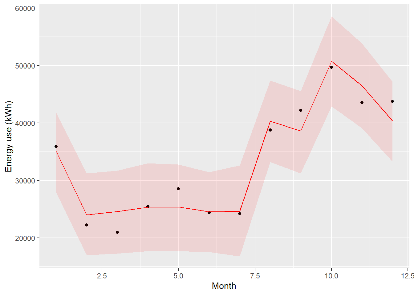

Figure 3.4: Comparison of model prediction and measurements in the pre period

We can calculate the usual metrics with the mean posterior prediction: coefficient of determination $R^2$, CV(RMSE), F-statistic…

residuals <- predict.mean - df.pre$use        # residuals
ssres <- sum(residuals^2)                     # sum of squared residuals
sstot <- sum((df.pre$use-mean(df.pre$use))^2) # total sum of squares

R2 <- 1 - ssres / sstot   # coefficient of determination
CVRMSE <- sqrt(ssres / nrow(df.pre)) / mean(df.pre$use)

print(paste("R2 =", R2))
print(paste("CV(RMSE) =", CVRMSE))

## [1] "R2 = 0.942258713375518"
## [1] "CV(RMSE) = 0.0696138062666448"

Prediction residuals should have low autocorrelation. This can be checked by the Durbin-Watson statistic, or with an autocorrelation plot:

acf(residuals)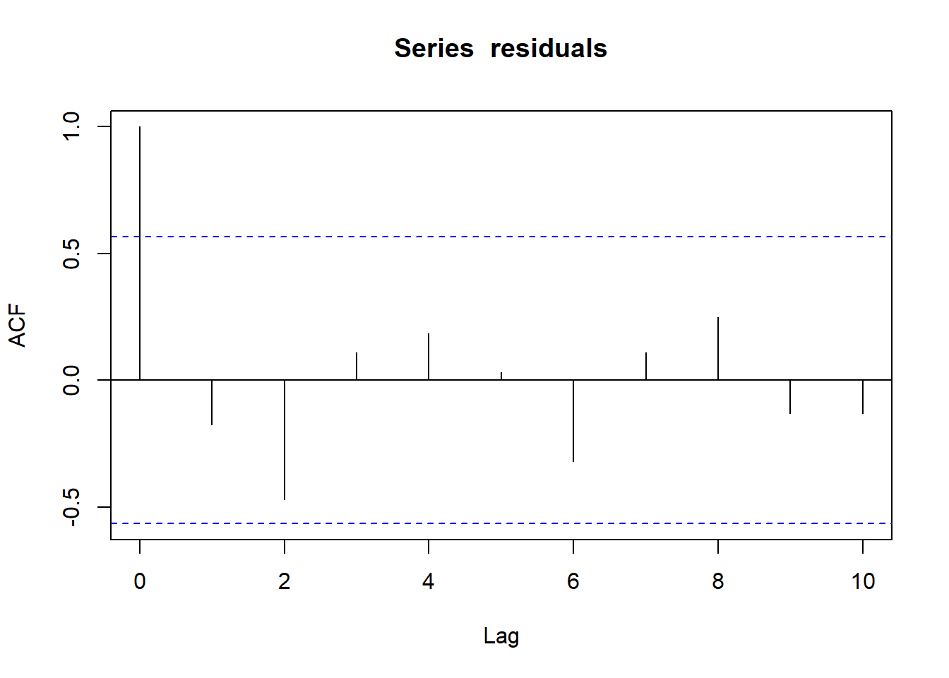

Figure 3.5: Autocorrelation function of the linear model residuals

We won’t elaborate much on this plot because we will focus on it in the next tutorial. In short, our simple linear model has low autocorrelation of residuals: this criterion is satisfied. However, the $R^2$ index is quite low: a significant part of the data’s variance is unexplained.

3.4.2 Checking model parameters

Individual parameter adequacy can be checked with the $t$-statistic or the $p$-value.

# Trace of all parameters and generated quantities
traces <- as.data.frame(fit)
# Only the parameters
traces.p <- traces %>% select('alpha', 'beta[1]', 'beta[2]', 'sigma')

# The t-statistic is the ratio of mean to standard deviation of parameters
t_stat <- colMeans(traces.p) / sapply(traces.p, sd)
# The p-value is easy to calculate from the t statistics
ptest <- 2*pt(-abs(t_stat), df=nrow(df.pre))

print(ptest)

##        alpha      beta[1]      beta[2]        sigma 
## 1.227476e-06 5.181084e-01 1.414004e-05 5.036975e-03

We can see that one $p$-value is over 0.05: beta[1] which is the regression coefficient of cooling degree-days.

The pairwise correlation of parameters is already visible on the pairplot shown earlier. There is a high correlation between them, which we can confirm quantitatively:

cor(traces.p)

##                alpha      beta[1]     beta[2]        sigma
## alpha    1.000000000 -0.861666528 -0.87471809  0.004493572
## beta[1] -0.861666528  1.000000000  0.76152890  0.009350584
## beta[2] -0.874718086  0.761528904  1.00000000 -0.015556055
## sigma    0.004493572  0.009350584 -0.01555605  1.000000000

3.5 Prediction of savings

We are only partially reassured on the adequacy of our model: the $R^2$ is not very high, one parameter may not be statistically significant, and parameters are quite correlated. The autocorrelation criterion is however satisfactory: this means that we may obtain unbiased estimates of energy savings, but they will probably have a high uncertainty.

Let’s fit a regular deterministic linear model, in order to compare its results with our Bayesian method:

fit2 <- lm(use ~ cdd + hdd, df.pre)
summary(fit2)

## 
## Call:
## lm(formula = use ~ cdd + hdd, data = df.pre)
## 
## Residuals:
##     Min      1Q  Median      3Q     Max 
## -3608.1 -1596.3  -225.6  1464.2  3636.7 
## 
## Coefficients:
##             Estimate Std. Error t value Pr(>|t|)    
## (Intercept)  22860.4     2136.0  10.702 2.03e-06 ***
## cdd            114.5      142.6   0.803    0.443    
## hdd            872.7      104.2   8.374 1.53e-05 ***
## ---
## Signif. codes:  0 '***' 0.001 '**' 0.01 '*' 0.05 '.' 0.1 ' ' 1
## 
## Residual standard error: 2681 on 9 degrees of freedom
## Multiple R-squared:  0.9421, Adjusted R-squared:  0.9292 
## F-statistic: 73.24 on 2 and 9 DF,  p-value: 2.702e-06

Yes, it is that simple.

The coefficients are the same as the Bayesian output. Without doing any model checking, we can expect the same conclusions.

Let’s now compare energy use predictions during the post-retrofit period, with the Bayesian method (in red) and the classical method (in blue):

# Model predictions during the "post" period
predict.post <- apply(la$predict_post, 2, quantile, probs=c(0.025, 0.5, 0.975))
# Predictions from an ordinary linear regression model
predict.2 <- predict(fit2, newdata = df.post, interval = "prediction", level=0.95)

xplot <- array(1:nrow(df.post))
ggplot(mapping = aes(x = xplot)) +
  geom_point(mapping = aes(y = df.post$use)) +
  geom_line(mapping = aes(y = predict.post[2,]), color='red') +
  geom_line(mapping = aes(y = predict.2[,1]), color='blue') +
  geom_ribbon(mapping = aes(ymin=predict.post[1,], ymax=predict.post[3,]), fill='red', alpha=0.1) +
  geom_ribbon(mapping = aes(ymin=predict.2[,2], ymax=predict.2[,3]), fill='blue', alpha=0.1)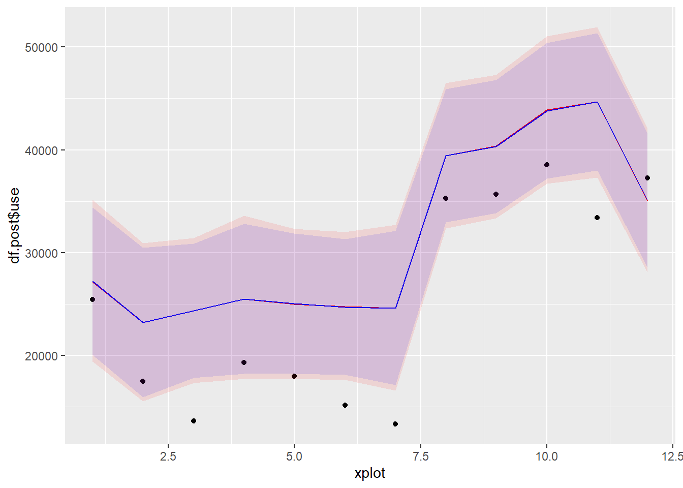

Figure 3.6: Model predictions and measurements in the post period

Predictions from both methods look almost exactly the same. Finally, let’s compare them on the basis of energy savings predictions. The following block generates a table containing the mean, lower and upper bounds of the 95% confidence interval, of predicted energy savings.

method <- c("bayesian", "classical")
# Mean savings
mean.savings <- c(mean(la$savings),
                  sum(predict.2[,1] - df.post$use))
# Lower and upper bounds of the 95% confidence interval of savings
lower.bound <- c(sum(predict.post[1,] - df.post$use),
                 sum(predict.2[,2] - df.post$use))
upper.bound <- c(sum(predict.post[3,] - df.post$use),
                 sum(predict.2[,3] - df.post$use)) 
svgs <- data.frame(method, mean.savings, lower.bound, upper.bound)

print(svgs)

##      method mean.savings lower.bound upper.bound
## 1  bayesian     75696.75  -12679.896    164579.1
## 2 classical     75564.54   -6385.537    157514.6

The mean savings estimate is the same with both method (with less than 1% difference), but there is some discrepancy on the lower and upper bounds of the 95% interval. I don’t believe there is a real reason for this gap since the specification of both models is identical. It is probably caused by the finite number of samples to properly approximate the tails of the posterior distribution.

3.6 Conclusion

In this tutorial, we showed how to perform Bayesian linear regression with Stan, in a typical M&V workflow. We estimate post-retrofit energy savings, adjusted to heating and cooling degree-days.

We showed that we obtain the same results (parameter estimates, model validation metrics, energy use predictions, savings uncertainty) with the Bayesian approach than the deterministic ordinary linear regression method. The Bayesian method seems much more complicated than the classical method, but we’ll show in the next tutorials that its workflow will remain the same regardless of model complexity, while the classical approach may no longer have simple solutions for estimating savings uncertainty.

2 Bayesian data analysis

4 Tutorial 2: increasing model complexity