1 Measurement and verification

This chapter and the next one are excerpts of the author’s larger website on building energy statistical modelling.

1.1 Intro to M&V and the IPMVP

Measurement and Verification (M&V) is the process of assessing savings caused by an Energy Conservation Measure (ECM). M&V is a crucial tool in the establishment of Energy Performance Contracts (EPC), which can be established on the basis of designed performance (building energy simulation), with an eventual uncertainty analysis and/or sensitivity analysis, or on the basis of measured energy consumption.

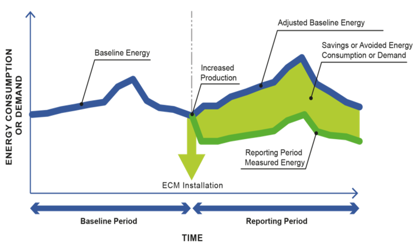
The International Performance Measurement and Verification Protocol (IPMVP) formalizes this process, and presents several options to conduct it. Savings are determined by comparing measured consumption or demand before and after implementation of a program, making suitable adjustments for changes in conditions.

An example of adjustment is, when estimating the energy savings delivered by an ECM, to substract its new energy consumption from the consumption that would have occurred if the building had stayed in the same situation in the weather conditions of the reporting period (adjusted baseline consumption). This requires a prediction model that can extrapolate the initial behaviour of the building by accounting for variable weather conditions. Other possible adjustments include changes in occupancy schedules. This is necessary to assess whether measured energy savings are caused by the ECM itself, or by changes in these influences.

Figure 1.1: The IPMVP provides guidelines on how to perform M&V

In the “avoided energy consumption” approach, savings are reported under the conditions of the reporting (post-retrofit) period. Alternatively, in the “normalized savings” approach, savings are calculated under a separate set of conditions, which requires fitting separate models for the pre- and post-ECM periods, and comparing their predictions in these new conditions.

The IPMVP presents several options, depending on whether the operation concerns an entire facility or a portion, and defines the notion of measurement boundary as the set of measurements that are relevant to determine savings (see Sec. 1.2 below).

• In order to verify the savings from a single equipment, and a measurement boundary can be drawn around it, the approach used is retrofit-isolation: IPMVP options A and B.
• If the purpose of reporting is to verify total facility energy performance, the approach is the whole-facility option C.
• In the IPMVP option D, savings are determined through simulation of the pre-ECM energy consumption rather than direct measurements. The simulation model is calibrated so that it predicts the energy and load that matches the post-ECM metered data.

1.2 Measurement and modelling boundaries

Most M&V options rely on the definition of a numerical model which reproduces the relationship between the variables monitored at the measurement boundary.

• The dependent variable \(y\), or model output, is a variable that we wish for a fitted model to be able to predict.
• The explanatory variables, or independent variables, are the model inputs by which we try to explain the evolutions of the dependent variable. Explanatory variables are denoted \(x\) in most regression models, or \(u\) in more complex hierarchical models where \(x\) may denote a latent variable instead.
• Some models have latent variables, which are unobserved and affect the dependent variable.

The IPMVP defines measurement boundaries as “notional boundaries drawn around equipment, systems or facilities to segregate those which are relevant to saving determination from those which are not. All Energy Consumption and Demand of equipment or systems within the boundary must be measured or estimated. […] Any energy effects occurring beyond the selected measurement boundary are called interactive effects. The magnitude of any interactive effects needs to be estimated or evaluated to determine savings associated with the ECMs.”

The same definition of boundaries work for simulations: a model must be defined so that its inputs and outputs are the measured independent and dependent variables, and all energy effects occurring within these boundaries are either fixed, or part of the list of parameters \(\theta\) that will be estimated by calibration.

Figure 1.2: Building energy models simulate the interactions between envelope, ambiance, HVAC systems and their controls, described by a finite set of parameters. The explanatory variables are related to the two conditions mentioned earlier: weather and occupants. The dependent variables are separate energy consumptions.

Typical modelling boundaries of building energy simulation (BES) resemble Fig. 1.2. The time-varying inputs provided by the user are weather files and occupancy profiles. Most of the time, the latter come from standard scenarios rather than measurement. Occupancy is understood by BES as a finite set of actions and influences: presence, temperature set-points, use of appliances. The model returns predictions of energy use, usually with a higher level of disaggregation (consumption of each system) than is easily available by measurement.

1.3 Error and uncertainty

Inverse problem theory can be summed up as the science of training models using measurements. The target of such a training is either to learn physical properties of a system by indirect measurements, or setting up a predictive model that can reproduce past observations.

The general principle of solving a system identification problem is to describe an observed phenomenon by a model allowing its simulation. Measurements \((\mathbf{x},\mathbf{y})\) are carried in an experimental setup: a building is probed for the quantities from which we wish to estimate its energy performance (indoor temperature, meter readings, climate, etc.) A model is defined as a mapping between some of the measurements set as input \(\mathbf{x}\) (boundary conditions, weather data) and some as output \(\mathbf{y}\). A numerical model is a mathematical formulation of the outputs \(f(x, \theta)\), parameterised by a finite set of variables \(\theta\). The most intuitive way to calibrate a model is to minimize an indicator such as the sum of squared residuals, in order to find the value of \(\theta\) that makes the model most closely match the data.

Ideally, the model is unbiased: it accurately describes the behaviour of the system, so that there exists a true value \(\theta^*\) of the parameter vector for which the model output reproduces the undisturbed value of observed variables. \[\begin{equation} y_k = f(x_k, \theta^*) + \varepsilon_k \tag{1.1} \end{equation}\] where \(\varepsilon\) denotes measurement error, i.e. the difference between the real process and its observed value \(y\). The most convenient assumption is that of additive noise, i.e. \(\varepsilon_k\) is a sequence of independent and identically distributed random variables.

In practice, \(\theta^*\) will never be reached exactly, but rather approached by an estimator \(\hat \theta\), because the entire process of estimating it from measurements is disturbed by an array of approximations:

• Experimental errors. The numerical data \((x,y)\) available for model calibration differs from the hypothetical outcome of the ideal, undisturbed physical system. Sensors may be intrusive, produce noisy measurements, may be poorly calibrated, have a finite precision and resolution…
• Numerical errors. The hypothesis of an unbiased model (Eq. (1.1)) states that there exists a parameter value \(\theta^*\) for which the model output is separated from the observations \(y\) only by a zero mean, Gaussian distributed measurement noise. It means that the model perfectly reproduces the physical reality, and the only perceptible error is due to the imperfection of sensors. This is exceedingly optimistic, especially in building energy simulation.

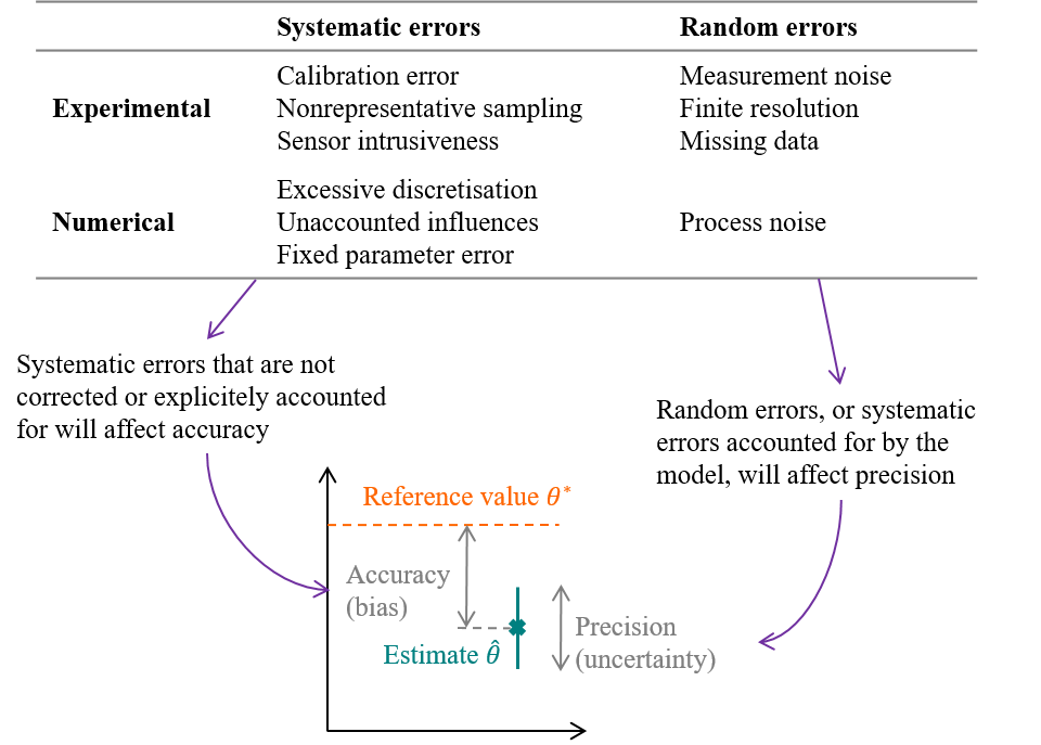
Figure 1.3: Errors and uncertainties on parameter estimation, caused by measurement and modelling errors

The Guide to the expression of Uncertainty in Measurement (GUM)(JCGM (2008)) then separates errors into a random component and a systematic component: systematic errors are errors which retain a non-zero mean if the measurement was repeated an infinite number of times under repeatability conditions. Systematic and random errors, whether they concern the measurement or the modelling procedures, will affect the estimation of a parameter \(\theta\) in terms of accuracy and precision. The figure above illustrates accuracy and precision in the case of estimating a parameter value \(\theta\), but the exact same terminology can be used if the purpose of the trained model is to predict the future values of a variable \(y\).

• The GUM defines uncertainty (of measurement) as the dispersion of the values that could reasonably be attributed to a measured quantity. Similarly, parameter estimates or model predictions come with an uncertainty, which quantifies their possible range of values caused by the random errors in the measurement and modelling processes. Precision is an indicator of low uncertainty, and can be conveyed by confidence intervals.
• On the other hand, accuracy is a measure of bias. It is the difference between the “true” value of the target variable and the mean of our estimation.

Biased estimates and predictions are the outcome of errors that have not been explicitely taken into account in the inverse problem. We tend to prefer low bias and high uncertainty, than high bias and low uncertainty: indeed, a high uncertainty suggests that the data were not sufficient to provide confident inferences, which incites caution when communicating the results.

This description of bias and uncertainty applies not only to the value of estimated model parameters, but to all predictions subsequently performed by the fitted model. In particular, this concerns the estimation of savings which are based on energy use predictions: our end goal is to obtain reliable (unbiased) inference of energy savings and their uncertainty. The motivation of this guide is to show that Bayesian methods are well suited for this goal.