Hamstad BM3

This script simulates the third exercise of the Hamstad benchmark package: transient heat and moisture transfer impacted by air flow through a lightweight wall.

Note that the external air pressure fluctuates on one side of the domain, and that its values are read from a .txt file which has two columns labeled Time (s) and DeltaP. This file is available in the hamopy/benchmarks folder

Script

import numpy  as np
import pandas as pd
import matplotlib.pylab as plt

# All things necessary to run the simulation
from hamopy import ham_library as ham
from hamopy.classes import Mesh, Boundary, Time
from hamopy.algorithm import calcul
from hamopy.postpro import evolution

# Choice of materials and geometry
from hamopy.materials.hamstad import BM3
mesh = Mesh(**{"materials"    : [BM3],
               "sizes"        : [0.2],
               "nbr_elements" : [40] })

# Boundary conditions
clim_file = 'BM3 climate.txt'
clim1 = Boundary('Fourier',**{"file"      : clim_file,
                              "time"      : "Time (s)",
                              "T"         : 293.15,
                              "HR"        : 0.7,
                              "h_t"       : 10,
                              "h_m"       : 2e-7,
                              "P_air"     : "DeltaP"})

clim2 = Boundary('Fourier',**{"T"         : 275.15,
                              "HR"        : 0.8,
                              "h_t"       : 10,
                              "h_m"       : 7.38e-12 })
clim = [clim1, clim2]

# Initial conditions
init = {'T'  : 293.15,
        'HR' : 0.95}

# Time step control
time = Time('variable',**{"delta_t"  : 900,
                          "t_max"    : 8640000,
                          "iter_max" : 12,
                          "delta_min": 1e-3,
                          "delta_max": 900 } )

# Calculation
results = calcul(mesh, clim, init, time)

# Post processing: what time and coordinate scales we wish to display the results on
data0 = pd.read_csv(clim_file, delimiter='\t')
t_out = np.array( data0['Time (s)'] )
x_out = [0.05, 0.1, 0.15, 0.17, 0.19]

# Use the evolution function to extract the temperature and humidity profiles
Temperature = np.column_stack([evolution(results, 'T', _, t_out) for _ in x_out])
Humidity = np.column_stack([evolution(results, 'HR', _, t_out) for _ in x_out])
MoistureContent = BM3.w(ham.p_c(Humidity, Temperature), Temperature)

# Plotting results
fig, ax = plt.subplots(2, 1)
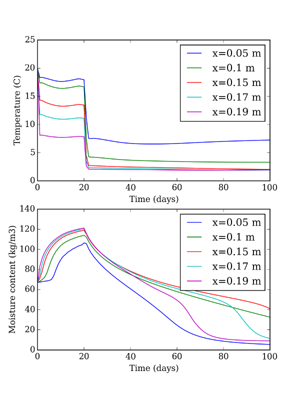
ax[0].plot(t_out / (24 * 3600), Temperature)
ax[0].set_xlabel('Time (days)')
ax[0].set_ylabel('Temperature (C)')
ax[0].legend(('x=0.05 m', 'x=0.1 m', 'x=0.15 m', 'x=0.17 m', 'x=0.19 m'))
ax[1].plot(t_out / (24 * 3600), MoistureContent)
ax[1].set_xlabel('Time (days)')
ax[1].set_ylabel('Moisture content (kg/m3)')
ax[1].legend(('x=0.05 m', 'x=0.1 m', 'x=0.15 m', 'x=0.17 m', 'x=0.19 m'))
plt.show()

Results